The document provides a tutorial on using gvSIG for geographic scripting, focusing on creating temperature reports for Germany from 1983 to 2005. It details steps for generating shapefiles, charts, and spreadsheets with temperature data, including code snippets for parsing, filtering, and visualizing data. Additionally, it acknowledges the sources and contributors that supported the creation of the tutorial.

1. GEOGRAPHIC SCRIPTING IN GVSIG
HALFWAY BETWEEN USER AND DEVELOPER
Geoinformation Research Group,
Department of Geography
University of Potsdam
21-25 November 2016
Andrea Antonello
PART 6: FROM GEO INTO YOUR REPORT

2. REPORTING UTILITIES
From within gvSIG it is possible also to create charts and documents.
Since those functionalities are not completely integrated into the
scripting engine, some tricky looking imports are required most of the
time. This should not scare the user that want's to generate simple
reports in batch mode.
In the following examples we will see how to produce charts and
spreadsheets.libreoffice

3. OBJECTIVE
Let's assume we have to write a report about how min and max average
temperature changed between 1983 and 2005 in Germany.
We want to create:
a shapefile containing polygons connected to the temperatures
a chart showing the monthly averages of min and max
a spreadsheet with the cleaned up dataset (ex. remove header)
The maps have to be in CRS EPSG:32632.
The necessary data can be found on the page of Surface meteorology and
Solar Energy maintained by NASA: https://eosweb.larc.nasa.gov/sse/

4. SUMMARY OF THE STEPS
Before we start, let's create a script with the comments of what we are
going to implement:
# parse temperature data and extract
# a list of information: [lat, lon, tempJan, tempFeb,...]
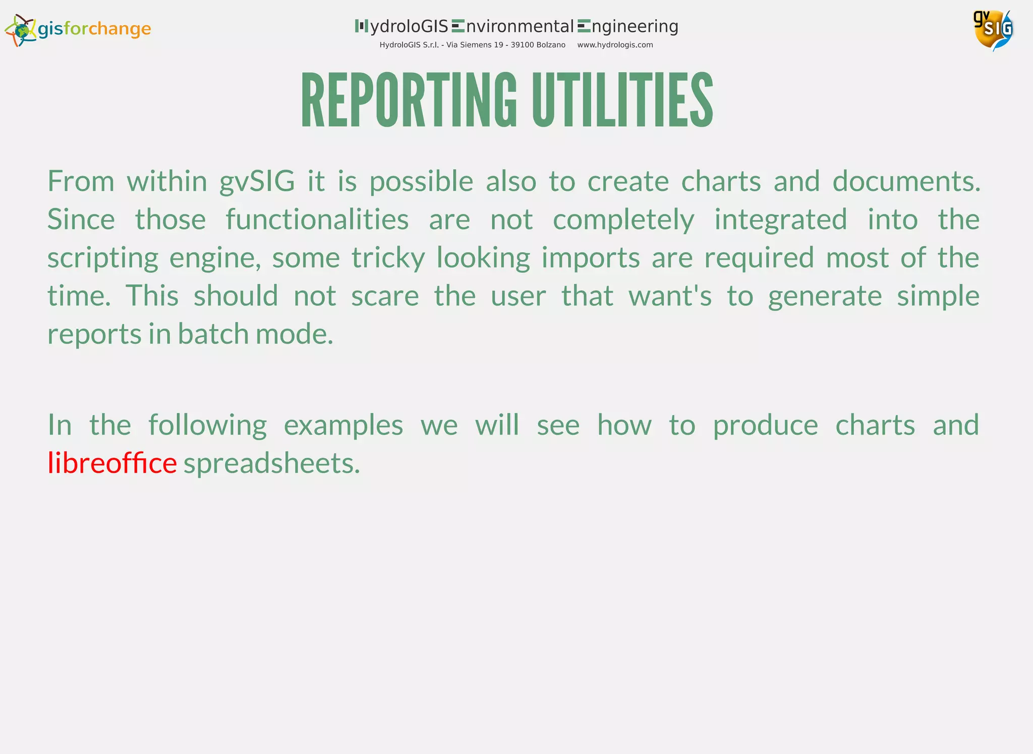
# create the shapefile
## get polygon of Germany
## filter only the data contained in the
## polygon of Germany
## create polygons with attached temperatures
## and write the features into the shapefile
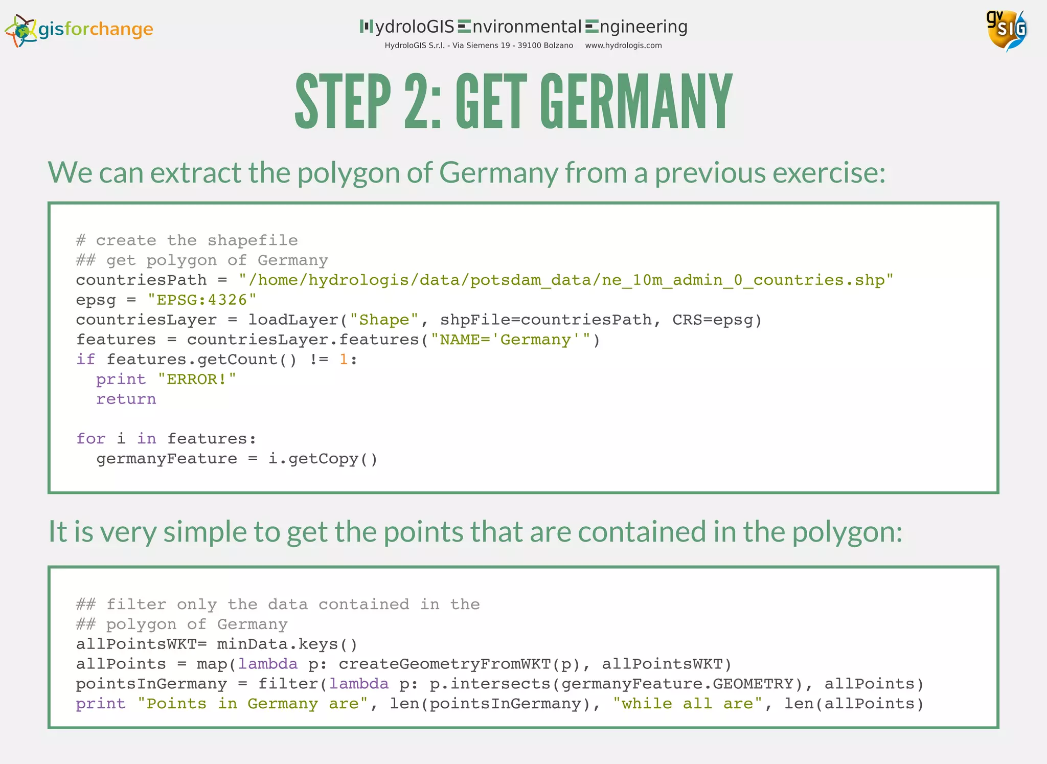
# create a chart of the average temperatures
# insert the parsed data into a spreadsheet

5. STEP 1: PARSE TEMPERATURE DATA
from gvsig import *
from gvsig.geom import *
def main(*args):
# parse temperature data and extract
# a dictionary {point: temperaturesList}
minPath = "/home/hydrologis/data/potsdam_data/22yr_T10MN"
dataFile = open(minPath, "r")
lines = dataFile.readlines()
dataFile.close()
data = {}
dataStarted = False
for line in lines:
if dataStarted or line.startswith("-90"):
dataStarted = True
lineSplit = line.split(" ")
lat = float(lineSplit[0])
lon = float(lineSplit[1])
pointLL = createPoint2D(lon, lat)
temperatures = []
for i in range(2, len(lineSplit)-1): # last is avg
temperatures.append(float(lineSplit[i]))
data[pointLL.convertToWKT()] = temperatures
print minData

6. STEP 1: PARSE TEMPERATURE DATA
def readData(path):
dataFile = open(path, "r")
lines = dataFile.readlines()
dataFile.close()
data = {}
dataStarted = False
for line in lines:
if dataStarted or line.startswith("-90"):
dataStarted = True
lineSplit = line.split(" ")
lat = float(lineSplit[0])
lon = float(lineSplit[1])
pointLL = createPoint2D(lon, lat)
temperatures = []
for i in range(2, len(lineSplit)-1): # last is avg
temperatures.append(float(lineSplit[i]))
data[pointLL.convertToWKT()] = temperatures
return data
def main(*args):
minPath = "/home/hydrologis/data/potsdam_data/22yr_T10MN"
maxPath = "/home/hydrologis/data/potsdam_data/22yr_T10MX"
minData = readData(minPath)
maxData = readData(maxPath)
To read also the max temperatures, let's do some code reuse:

7. STEP 2: GET GERMANY
# create the shapefile
## get polygon of Germany
countriesPath = "/home/hydrologis/data/potsdam_data/ne_10m_admin_0_countries.shp"
epsg = "EPSG:4326"
countriesLayer = loadLayer("Shape", shpFile=countriesPath, CRS=epsg)
features = countriesLayer.features("NAME='Germany'")
if features.getCount() != 1:
print "ERROR!"
return
for i in features:
germanyFeature = i.getCopy()
We can extract the polygon of Germany from a previous exercise:
It is very simple to get the points that are contained in the polygon:
## filter only the data contained in the
## polygon of Germany
allPointsWKT= minData.keys()
allPoints = map(lambda p: createGeometryFromWKT(p), allPointsWKT)
pointsInGermany = filter(lambda p: p.intersects(germanyFeature.GEOMETRY), allPoints)
print "Points in Germany are", len(pointsInGermany), "while all are", len(allPoints)

8. STEP 3: WRITE THE SHAPEFILE
## create polygons with attached temperatures
## and write the features into the shapefile
# create the transform between the original crs and the required
newEpsg = "EPSG:32632"
crs = getCRS(epsg)
newCrs = getCRS(newEpsg)
transform = crs.getCT(newCrs)
# create the new shapefile and set the editing mode
schema = createFeatureType()
schema.append("min", "DOUBLE", 8)
schema.append("max", "DOUBLE", 8)
schema.append("GEOMETRY", "GEOMETRY")
schema.get("GEOMETRY").setGeometryType(POLYGON, D2)
shape = createShape(schema, prefixname="minmaxtemperatures", CRS=newEpsg)
shape.edit()
First prepare the re-projection transformation and the output shapefile

9. STEP 3: WRITE THE SHAPEFILE
for point in pointsInGermany:
x = point.x
y = point.y
# points all represent the lower left corner
# create the polygon considering that
pts = [[x,y],[x,y+1],[x+1,y+1],[x+1,y],[x,y]]
polygon = createPolygon2D(pts)
# reproject the polygon
polygon.reProject(transform)
# use the point's WKT as key to get the temperature data
# from the dictionary
minAvg = sum(minData[point.convertToWKT()])/12.0
maxAvg = sum(maxData[point.convertToWKT()])/12.0
shape.append(min=minAvg, max=maxAvg, GEOMETRY=polygon)
shape.commit()
Then, in the main loop, reproject, average and write:

10. STEP 3: WRITE THE SHAPEFILE
# create an interval legend on the min values
intervalLegend = VectorialIntervalLegend(POLYGON)
intervalLegend.setStartColor(getColorFromRGB(0,0,255))
intervalLegend.setEndColor(getColorFromRGB(255,0,0))
intervalLegend.setIntervalType(1)
store = shape.getFeatureStore()
intervals = intervalLegend.calculateIntervals(store, "MIN", 5, POLYGON)
intervalLegend.setIntervals(intervals)
shape.setLegend(intervalLegend)
newview = currentProject().createView("Germany View")
newview.setProjection(getCRS(newEpsg))
newview.addLayer(shape)
newview.addLayer(countriesLayer)
newview.showWindow()
newview.centerView(shape.fullEnvelope)
Style and load the data. Also load the countries layer to check the result.
Since (as we already know) the countries layer will be messy outside the
32632 zone, also zoom to the area of Germany:

11. INTERMEDIATE CHECK
A this point the script, if run, should produce something like this
(countries are styled to only show the borders)

12. STEP 4: CHART THE DATA
Charts can be created through the use of the project.
Charting in not exactly integrated in the scripting engine, so it requires
for the user to import a whole pile of modules.
The following are the ones we will make use of in the example:
jfreechart
from org.jfree.chart import ChartFactory
from org.jfree.chart import ChartFrame
from org.jfree.data.xy import XYSeriesCollection
from org.jfree.data.xy import XYSeries
from org.jfree.chart.plot.PlotOrientation import *

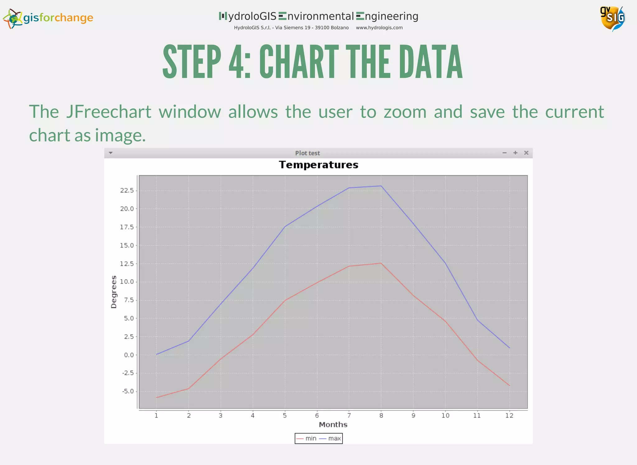
13. STEP 4: CHART THE DATA
Let's pick the first point of the list of points inside Germany:
# create a chart of the average temperatures
chartPoint = pointsInGermany[0]
minTemperaturesList = minData[chartPoint.convertToWKT()]
maxTemperaturesList = maxData[chartPoint.convertToWKT()]
Then create the XY chart series, fill them with the temperature data per
month and add them to a series collection:
dataset = XYSeriesCollection()
seriesMin = XYSeries("min")
seriesMax = XYSeries("max")
for i in range(0, 12):
month = i + 1
seriesMin.add(month, minTemperaturesList[i])
seriesMax.add(month, maxTemperaturesList[i])
dataset.addSeries(seriesMin)
dataset.addSeries(seriesMax)

14. STEP 4: CHART THE DATA
Finally create the chart and display it in a windows:
chart = ChartFactory.createXYLineChart(
"Temperatures", # chart title
"Months", # x axis label
"Degrees", #y axis label
dataset,
VERTICAL, # orientation
True, # include legend
True, # tooltips?
False # URLs?
)
# show the chart in a window
frame = ChartFrame("Plot test", chart);
frame.pack();
frame.setVisible(True);

15. STEP 4: CHART THE DATA
The JFreechart window allows the user to zoom and save the current
chart as image.

16. STEP 5: SPREADSHEETS
To create an modify spreadsheets gvSIG makes use of the
project.
On its homepage a
. In there it is possible to find all the functions that are
used in the next example.
In the same way as for the charting part, also the spreadsheet part needs
some dedicated import statements:
jopendocument
section is dedicated to the programmer
documentation
from java.io import File
from org.jopendocument.model import OpenDocument
from org.jopendocument.dom.spreadsheet import SpreadSheet
from org.jopendocument.dom import OOUtils

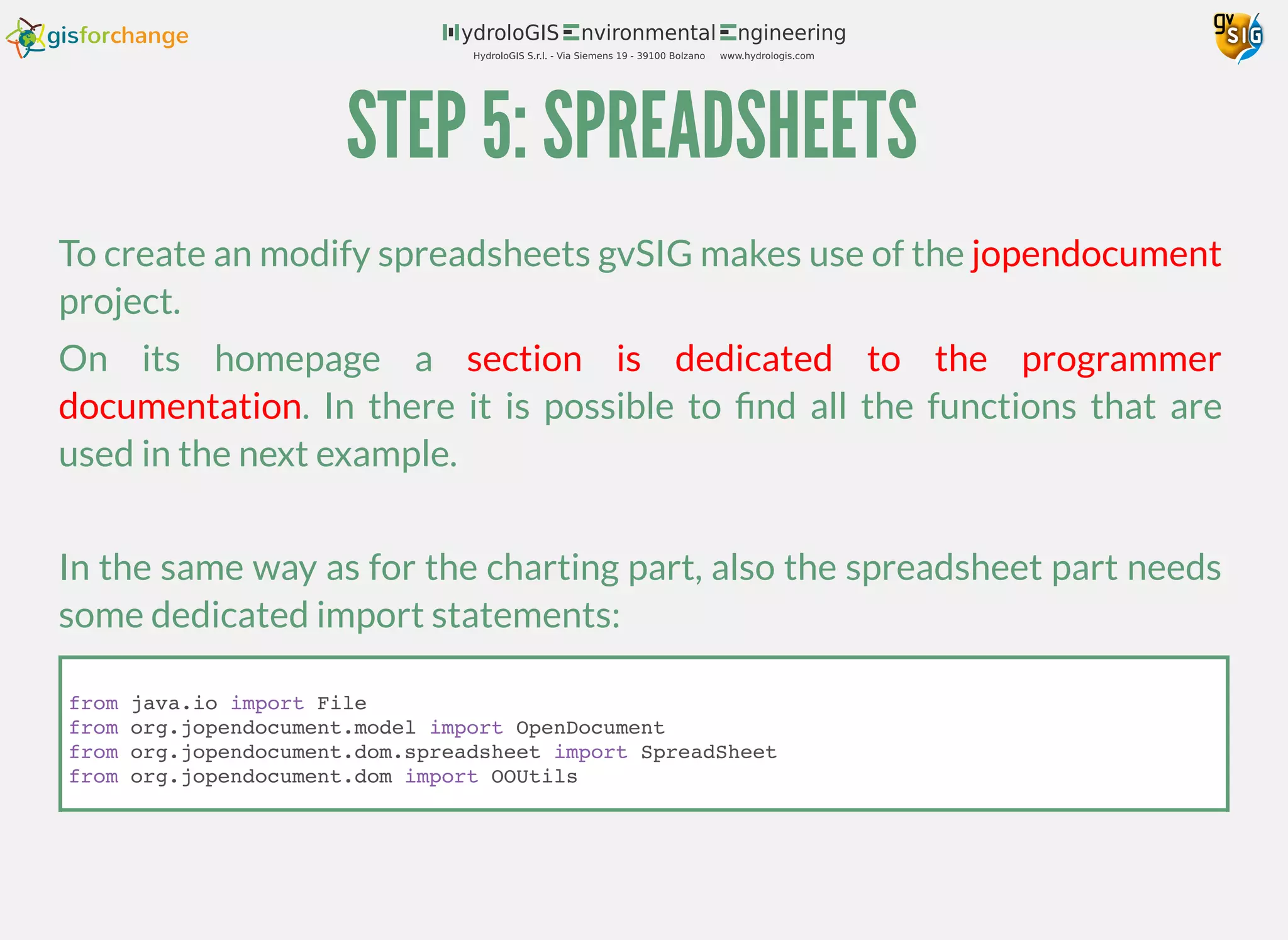
17. STEP 5: SPREADSHEETS
It is simple to set values in the cells by using the column and row as one
would do with a matrix:
# write the header row in both sheets
header = ["lat", "lon", "jan", "feb", "mar", "apr", "may",
"jun", "jul", "aug", "sep", "oct", "nov", "dec"]
for i, value in enumerate(header):
minSheet.setValueAt(value, i, 0)
maxSheet.setValueAt(value, i, 0)
Once the imports are in place, it is possible to create a new spreadsheet
and add two sheets to it for the min and max table values:
# insert the parsed data into a spreadsheet
spreadsheetPath = "/home/hydrologis/data/potsdam_data/data_test.ods"
# create a spreadsheet
spreadSheet = SpreadSheet.create(2, 100, 70000)
minSheet = spreadSheet.getSheet(0)
minSheet.setName("MIN")
maxSheet = spreadSheet.getSheet(1)
maxSheet.setName("MAX")

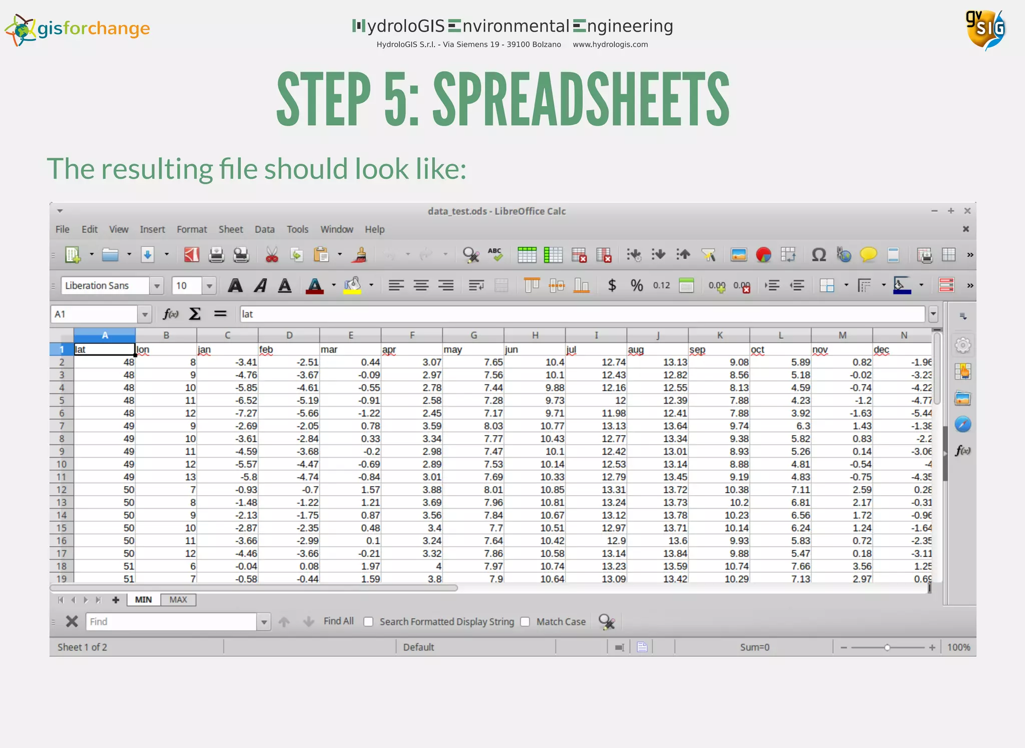
18. STEP 5: SPREADSHEETS
Then we can loop the ranges of lat and lon in order to have an ordered list
of only the values inside Germany:
row = 0
for lat in range(-90, 89):
for lon in range(-180, 179):
p = createPoint2D(lon, lat)
if p in pointsInGermany:
row += 1
minSheet.setValueAt(lon, 1, row)
minSheet.setValueAt(lat, 0, row)
maxSheet.setValueAt(lon, 1, row)
maxSheet.setValueAt(lat, 0, row)
minTemperaturesList = minData[p.convertToWKT()]
maxTemperaturesList = maxData[p.convertToWKT()]
for i, t in enumerate(minTemperaturesList):
col = i + 2
minSheet.setValueAt(t, col, row)
maxSheet.setValueAt(maxTemperaturesList[i], col, row)
Finally, save and open the file:
outputFile = File(spreadsheetPath)
OOUtils.open(spreadSheet.saveAs(outputFile))

19. STEP 5: SPREADSHEETS
The resulting file should look like:

20. <license>
This work is released under Creative Commons Attribution Share Alike (CC-BY-SA).
</license>
<sources>
Much of the knowledge needed to create this training material has been produced
by the sparkling knights of the
<a href="http:www.osgeo.org">Osgeo</a>,
<a href="http://tsusiatsoftware.net/">JTS</a>,
<a href="http://www.jgrasstools.org">JGrasstools</a> and
<a href="http:www.gvsig.org">gvSIG</a> communities.
Their websites are filled up with learning material that can be use to grow
knowledge beyond the boundaries of this set of tutorials.
Another essential source has been the Wikipedia project.
</sources>
<acknowledgments>
Particular thanks go to those friends that directly or indirectly helped out in
the creation and review of this series of handbooks.
Thanks to Antonio Falciano for proofreading the course and Oscar Martinez for the
documentation about gvSIG scripting.
</acknowledgments>
<footer>
This tutorial is brought to you by <a href="http:www.hydrologis.com">HydroloGIS</a>.
<footer>