This document discusses period-doubling bifurcations and the route to chaos in an area-preserving discrete dynamical system. It highlights two objectives: 1) Evaluating period-doubling bifurcations using computer programs as the system parameter p is varied, obtaining the Feigenbaum universal constant and accumulation point beyond which chaos occurs; and 2) Confirming periodic behaviors by plotting time series graphs. The document provides background on Feigenbaum universality and describes the specific area-preserving map studied. It outlines the numerical method used to obtain periodic points via Newton's recurrence formula and describes applying this to the map's Jacobian matrix.

1. I nternational Journal Of Computational Engineering Research (ijceronline.com) Vol. 2 Issue. 7
Route to Chaos in an Area-preserving System
Dr. Nabajyoti Das
Assistant Professor, Depart ment of Mathematics Jawaharlal Nehru Co llege, Bo ko -781123
District : Kamrup, State: Assam, Country: India
Abstract:
Th is paper highlights two important objectives on a two-dimensional area-preserving discrete dynamical system:
E( x, y)  ( y  px  (1  p) x 2 , x  y  px  (1  p) x 2 ) ,
where p is a tunable parameter. Firstly, by adopting suitable computer programs we evaluate period-doubling:
period 1  period 2  period 4  ...  period 2 k  ...  chaos
bifurcations, as a universal route to chaos, for the periodic orbits when the system parameter p varied and obtain the
Feigenbaum universal constant = 8.7210972…, and the accumulation point  = 7.533284771388…. beyond which
chaotic region occurs.. Secondly, the periodic behaviors of the system are confirmed by plotting the time series graphs.
Key Words: Period-doubling bifurcations/ Periodic orbits / Feigenbaum universal constant / Accumulation point /
Chaos / Area-preserving system
2010 AMS Classificat ion: 37 G 15, 37 G 35, 37 C 45
1. Introduction
The initial universality discovered by Mitchell J. Feigenbaum in 1975 has successfully led to discover that large
classes of nonlinear systems exhib it transitions to chaos which are universal and quantitatively measurable. If X be a
suitable function space and H, the hypersurface of co-d imension 1 that consists of the maps in X having derivative -1 at
the fixed point, then the Feigenbaum uni versality is closely related to the doubling operator, F acting in X defined by
(F )( x)   ( ( 1 x))  X
where  = 2.5029078750957… , a universal scaling factor. The principal properties of F that lead to universality are
*
(i) F has a fixed point x ;
(ii) The linearised transformation DF ( x * ) has only one eigenvalue  greater than 1 in modulus; here  =
4.6692016091029…
(iii) The unstable man ifold corresponding to  intersects the surface H transversally; In one dimensional case, thes e
properties have been proved by Lanford [2, 10].
Next, let X be the space of two parameter family of area- preserving maps defined in a domain U   2 , and Y, the
space of two parameter family o f maps defined in the same domain having not necessarily constant Jacobian. Then Y
contains X. In area- preserving case, the Doubling operator F is defined by
F   1 2  ,
where  :  2   2 , ( x, y)  (x, y) is the scaling transformation. Here  and  are the scaling factors;
numerically we have   0.248875... and   0.061101... In the area p reserving case, Feigenbaum constant,  =
8.721097200….. Furthermore, one of his fascinating discoveries is that if a family  presents period doubling
 n   n1
bifurcations then there is an infinite sequence {  n } of bifurcation values such that   lim   , where
n   n1   n
 is a universal number already mentioned above. Moreover, his observation suggests that there is a universal size -
d
scaling in the period doubling sequence designated as the Feigenbaum   value,   lim n  2.5029... where d n
n  d n1
is the size of the bifurcation pattern of period 2 n just before it g ives birth to period 2 n1 [1, 6-8].
Issn 2250-3005(online) November| 2012 Page 38

2. I nternational Journal Of Computational Engineering Research (ijceronline.com) Vol. 2 Issue. 7
The birth and flowering of the Feigenbaum universality with numerous non -linear models has motivated me to wrire this
paper.
2. Our Nonlinear Map and the Feigenbaum Universality:
Our concerned map:
E( x, y)  ( y  px  (1  p) x 2 , x  y  px  (1  p) x 2 ) (1.1)
where p is a tunable parameter. The Jacobian of E is the unity, so is area-preserving.
The map has one fixed point other than (0,0) whose coordinates is given by
3 p 6  2 p
x ,y 
1  p 1 p
Fro m this one finds that E has no fixed point if p = 1. In this context, we also wish to point out that the stability
theory is intimately connected with the Jacobian matrix of the map, and that the trace of the Jacobian matrix is the sum
of its eigenvalues and the product of the eigenvalues equal the Jacobian determinant. For a particular value of p, the map
E depends on the real parameter p, and so a fixed point x s of this map depends on the parameter value p, i.e.
x s  x s ( p) . No w, first consider the set, U  (,3)  (7,) .
The fixed point x s remains stable for all values of p lying in U and a stable periodic trajectory of period-one appears
around it. This means, the two eigenvalues
 5   7  p  3  p (1  p)  6 p  p 2
1  ,
2(1  p)
 5   7  p  3  p (1  p)  6 p  p 2
2 
2(1  p)
of the Jacobian mat rix:
 p  2(1  p) x  1
J 
1  p  2(1  p) x  1
at x s remains less than one in modulus and consequently, all the neighbouring points (that is, points in the
domain of attraction) are attracted towards x s ( p) ), p lying in U. If we now begin to increase the value of p, then it
happens that one of the eigenvalues starts decreas ing through –1 and the other remains less than one in modulus . When
p = 7, one of the eigenvalues becomes –1 and then x s loses its stability, i.e. p1  7 emerg ing as the first bifurcati on
value of p. Again, if we keep on increasing the value of p the point x s ( p) becomes unstable and there arises around it
two points, say, x 21 ( p) and x 22 ( p) forming a stable periodic trajectory of period-two. A ll the neighbouring points
except the stable manifold of x s ( p) are attracted towards these two points . Since the period emerged becomes double,
the previous eigenvalue which was –1 becomes +1 and as we keep increasing p, one of the eigenvalues starts decreasing
fro m +1 to –1.Since the trace is always real, when eigenvalues are complex, they are conjugate to each other moving
n
along the circle of radius pe , where p e = p 2 is the effective Jacobian, in the opposite directions . When we reach a
certain value of p, we find that one of the eigenvalues of the Jacobian of E2 (because of the chain rule of differentiation, it
does not matter at which periodic point one evaluates the eigenvalues) becomes -1, indicating the loss of stability of the
periodic trajectory of period 2. Thus, the second bifurcation takes place at this value p 2 of p. We can then repeat the same
arguments, and find that the periodic trajectory of period 2 becomes unstable and a periodic trajectory of period 4
appears in its neighbourhood. This phenomenon continues upto a particular value o f p say p 3 (p), at wh ich the periodic
trajectory of period 4 losses its stability in such a way that one of the eigenvalues at any of its periodic points become –1,
and thus it gives the third bifurcat ion at p 3 (p). Increasing the value further and fu rther, and repeating the same argu ments
we obtain a sequence {p n (p)} as bifurcation values for the parameter p such that at pn (p) a periodic trajectory of period
2n arises and all periodic trajectories of period 2m(m<n) remain unstable. The sequence {pn (p)} behaves in a universal
manner such that p  (p)- p n (p)}  c(p )-n , where c(p) is independent of n and  and is the Feigenbaum uni versal
constant. Since the map has constant Jacobian 1(unity), we have the conservative case, i.e. the preservation of area and
in this case  equals 8.721097200…. Furthermore, the Feigenbaum theory says that the our map E at parameter = p (p)
Issn 2250-3005(online) November| 2012 Page 39

3. I nternational Journal Of Computational Engineering Research (ijceronline.com) Vol. 2 Issue. 7
has an invariant set S of Cantor type encompassed by infinitely many unstable periodic orbits of period 2n (n = 0, 1, 2,…),
and that all the neighbouring points except those belonging to these unstable orbits and their stable manifolds are
attracted to S under the iterations of the map E.
3. Numerical Method For Obtaining Periodic Points [2]:
Although there are so many sophisticated numerical algorithms available, to find a periodic fixed point, we have
found that the Newton Recurrence formula is one of the best numerical methods with neglig ible error for our purpose.
Moreover, it gives fast convergence of a periodic fixed point.
The Newton Recurrence formu la is
x n 1  x n  Df (x n ) 1 f (x n ),
where n = 0,1,2,… and Df ( x) is the Jacobian of the map f at the vector x . We see that this map f is equal to E k  I in
our case, where k is the appropriate period. The Newton formu la actually gives the zero(s) of a map, and to apply this
numerical tool in our map one needs a number of recurrence formu lae which are given below.
Let the in itial point be ( x0 , y 0 ),
Then,
E( x0 , y 0 )  ( y 0  px0  (1  p) x0 , x0  y 0  px0  (1  p) x0 )  ( x1 , y1 )
2 2
E 2 ( x0 , y 0 )  E ( x1 , y1 )  ( x 2 , y 2 )
Proceeding in this manner the following recurrence formu la fo r our map can be established.
x n   y n1  px n1  (1  p) x n1 , and y n   y n1  pxn1  (1  p) xn1 ,
2 2
where n = 1,2,3…
Since the Jacobian of Ek ( k times iteration of the map E ) is the product of the Jacobian of each iteration of the map, we
proceed as follows to describe our recurrence mechanism for the Jacobian matrix.
The Jacobian J 1 for the transformation
E( x0 , y0 )  ( y0  px0  (1  p) x0 , x0  y0  px0  (1  p) x0 ) is
2 2
 p  2(1  p) x0  1  A1 B1 
J1    
1  p  2(1  p) x
 0  1  C1
  D1 

where A1  p  2(1  p) x0 , B1  1, C1  1  p  2(1  p) x0 , D1  1.
Next the Jacobian J2 for the transformat ion
E2 ( x0 , y0 ) = ( x2 , y2 ), is the product of the Jacobians for the transformations
E ( x1 , y1 )  ( y1  px1  (1  p) x1 , x1  y1  px1  (1  p) x1 ) and
2 2
E ( x0 , y0 )  ( y0  px0  (1  p) x0 , x0  y0  px0  (1  p) x0 ).
2 2
So, we obtain
 p  2(1  p) x1  1 A1 B1   A2 B2 
J2  
1  p  2(1  p) x   ,
 1  1 C1
 D1   C 2
  D2 

where A2  [ p  2(1  p) x1 ] A1  C1 , B2  [ p  2(1  p) x1 ]B1  D1 ,
C2  [1  p  2(1  p) x1 ] A  C1 , D2  [1  p  2(1  p) x1 ]B1  D1.
1
m
Continuing this process in this way, we have the Jacobian for E as
A Bm 
Jm   m
C 

 m Dm 
with a set of recursive formula as
Am  [ p  2(1  p) xm1 ] Am1  Cm1 , Bm  [ p  2(1  p) xm1 ]Bm1  Dm1 ,
Cm  [ p  2(1  p) xm1 ] Am1  Cm1 , Dm  [ p  2(1  p) xm1 ]Bm1  Dm1 ,
(m = 2, 3, 4, 5…).
Since the fixed point of this map E is a zero of the map
G( x, y)  E( x, y)  ( x, y),
the Jacobian of G (k ) is given by
Issn 2250-3005(online) November| 2012 Page 40

4. I nternational Journal Of Computational Engineering Research (ijceronline.com) Vol. 2 Issue. 7
 A 1 Bk 
Jk  I   k
 C 
 k Dk  1

1  Dk  1 Bk 
Its inverse is ( J k  I ) 1   ,
  Ck
 Ak  1

where   ( Ak  1)( Dk  1)  Bk Ck ,
the Jacobian determinant. Therefo re, Newton‟s method gives the following recurrence formu la in order to yield a
periodic point ofEk
( D  1)( xn  xn )  Bk ( y n  y n )
ˆ ˆ
xn1  xn  k

(C k )( xn  xn )  ( Ak  1)( y n  y n )
ˆ ˆ
y n1  y n  ,

where E k (x n )  ( xn , y n ).
ˆ ˆ
4. Numerical Methods For Finding Bifurcation Values [2, 4 ]:
k
First of all, we recall our recurrence relations for the Jacobian matrix of the map E described in the Newton‟s
method and then the eigenvalue theory gives the relation Ak  Dk  1  Det ( J k ) at the bifurcation value. Again the
Feigenbaum theory says that
p  pn
p n2  p n1  n1 (1.2)

where n = 1,2,3,… and  is the Feigenbaum universal constant.
In the case of our map, the first two bifurcat ion values p 1 and p 2 can be evaluated.
Furthermore, it is easy to find the periodic points for p 1 and p 2. We note that if we put I  Ak  Dk  1  Det ( J k ) , then
I turns out to be a function of the parameter p . The bifurcation value of p of the period k occurs when I(p) equals zero.
This means, in order to find a bifurcation value of period k, one needs the zero of the function I(p), which is given by the
Secant method,
I ( pn )( pn  pn 1 )
pn 1  pn  .
I ( pn )  I ( pn1 )
Then using the relation (1.2), an approximate value 
p3 of p3 is obtained. Since the Secant method needs two initial
values, we use 
p3 and a slightly larger value, say,  4
p3  10 as the two initial values to apply this method and
ultimately obtain p3 . In like manner, the same procedure is emp loyed to obtain the successive bifurcation values
p4 , p5 ,... etc. to our requirement.
For finding periodic points and bifurcation values for the map E, above numerical methods are used and consequently,
the following Period-Doubling Cascade : Table 1.1, showing bifurcation points and corresponding periodic points , are
obtained by using suitable computer programs :
Table 1.1
Period One of the Periodic points Bifurcation Pt.
1 (x=0.666666666666...., y= -1.333333333333....) p1=7.00000000000
2 (x= -0.500000000003..., y= -1.309016994376...) p2=7.47213595500
4 (x= -0.811061640408 ..., y= -1.273315586957...) p3=7.525683372…
8 (x=-0.813878975794 ..., y= -1.275108054848...) p4=7.531826966…
16 (x=-0.460474775277...,y= -1.273990103300...) p5=7.532531327…
32 (x=-0.46055735696 ..., y= -1.274198905689...) p6=7.532612093…
64 (x=-0.54742669886 ..., y= -1.356526357634...) p7=7.532621354…
128 (x=-0.547431479795 ..., y= -1.356530832564...) p8=7.532636823…
… … … … … … ..
Issn 2250-3005(online) November| 2012 Page 41

5. I nternational Journal Of Computational Engineering Research (ijceronline.com) Vol. 2 Issue. 7
For the system (1.1), the values of  are calculated as follows:
p  p1 p  p2
1  2  8.8171563807015..., 2  3  8.715976842041...,
p3  p 2 p 4  p3
p 4  p3 p  p4
3   8.722215813427..., 4  5  8.721026780948...,
p5  p 4 p 6  p5
and so on.
The ratios tend to a constant as k tends to infinity: mo re formally
 b  bk 1 
lim  k     8.7210972...
k   bk 1  bk 
And the above table confirms that the „universal‟ Feigenbaum constant δ = 8.7210972…
is also encountered in this area-preserving two-dimensional system.
The accumu lation point p  can be calculated by the formula
1
p  ( p2  p1 )  p2 ,
 1
where δ is Feigenbaum constant, it is found to be 7.533284771388…. ., beyond which the system (1.1) develops chaos.
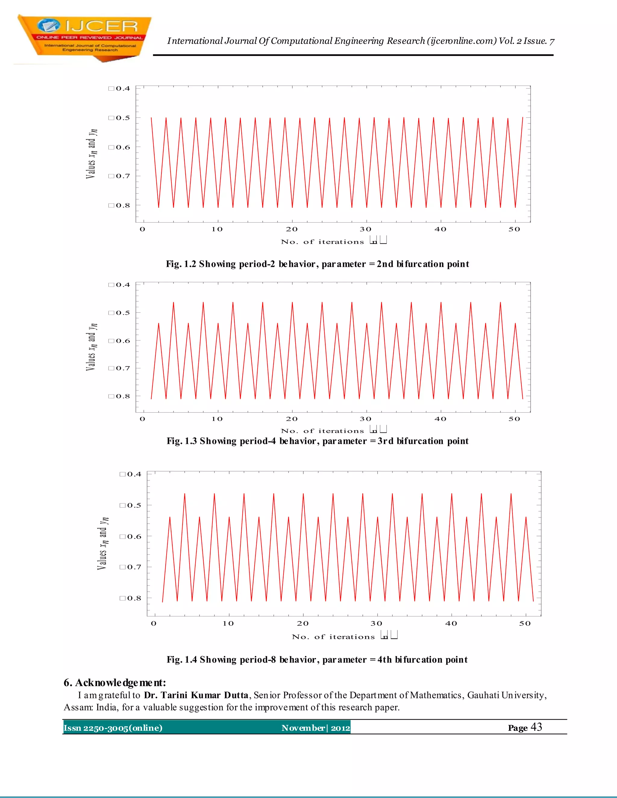
5. Time Series Graphs [3]
The key theoretical tool used for quantifying chaotic behavior is the notion of a time series of data for the
system [9]. A t ime series is a chronological sequence of observations on a particular variable. Usually the observations
are taken at regular intervals. The system (1.1) giv ing the difference equations:
xn1   y n  pxn  (1  p) xn , y n1  xn  y n  pxn  (1  p) xn , n  0,1,2,...
2 2
(1.3)
On the horizontal axis the number of iterat ions („time‟) are marked, that on the vertical axis the amp litudes are given for
each iteration. The system (1.3) exhib is the follo wing discrete time series graphs for the values of xn and yn , plotted
together, showing the existences of periodic orb its of periods 2k , k = 0, 1, 2,…, at d ifferent parameter
0.50
0.55

Values xn and yn
0.60
0.65
0.70
0.75

0.80
0 10 20 30 40 50
No. of iterations n
values.
Fig. 1 Showi ng period-1 behavi or, parameter = 1st bifurcati on poi nt
Issn 2250-3005(online) November| 2012 Page 42

6. I nternational Journal Of Computational Engineering Research (ijceronline.com) Vol. 2 Issue. 7
0.4
0.5
Values xn and yn
0.6
0.7
0.8
0 10 20
No. of iterat ions
30

n
40 50
Fig. 1.2 Showing period-2 behavior, parameter = 2nd bi furcation point
 .4
0
 .5
0
Values xn and yn
 .6
0
 .7
0
 .8
0
0 10 20 30
N o . o f i t erat i o n s 
n
40
Fig. 1.3 Showing period-4 behavior, parameter = 3rd bifurcation point
50
0.4
0.5
Values xn and yn
0.6
0.7
0.8
0 10 20
No. of iterations
30

n
40 50
Fig. 1.4 Showing period-8 behavior, parameter = 4th bi furcation point
6. Acknowledgement:
I am g rateful to Dr. Tarini Kumar Dutta, Sen ior Professor of the Depart ment of Mathematics, Gauhati Un iversity,
Assam: India, for a valuable suggestion for the improvement of this research paper.
Issn 2250-3005(online) November| 2012 Page 43

7. I nternational Journal Of Computational Engineering Research (ijceronline.com) Vol. 2 Issue. 7
7. References:
[1] Deveney R.L. “ An introduction to chaotic dynamical systems ”, Addison-Wiseley Publishing Co mpany,Inc
[2] Davie A. M . and Dutta T. K., “Period-doubling in Two-Parameter Families,” Physica D, 64,345-354, (1993).
[3] Das, N. and Dutta, N., “ Time series analysis and Lyapunov exponents for a fi fth degree chaotic map ”, Far East
Journal of Dynamical Systems Vo l. 14, No. 2, pp 125- 140, 2010
[4] Das, N., Sharmah, R. and Dutta, N., “Period doubling bifurcation and associated universal properties in the
Verhulst population model”, International J. of Math. Sci. & Engg. Appls. , Vo l. 4 No. I (March 2010), pp. 1 -14
[5] Dutta T. K. and Das, N., “Period Doubling Route to Chaos in a Two-Dimensional Discrete Map”, Global
Journal of Dynamical Systems and Applications, Vol.1, No. 1, pp 61 -72, 2001
[6] Feigenbaum .J M, “Quantitative Universality For Nonlinear Transformations” Journal of Statistical Physics, Vol.
19, No. 1,1978.
[7] Chen G. and Dong X., Fro m Chaos to Order: Methodologies, Perspectives and Applications, World Scientific,
1998
[8] Peitgen H.O., Jurgens H. and Saupe D. , “ Chaos and Fractal”, New Frontiers of Science, Springer Verlag, 1992
[9] Hilborn R. C “Chaos and Nonlinear Dynamics”,second edition, Oxford University
Press, 1994
[10] Lanford O.E. III, “A Co mputer-Assisted Proof of the Feigenbaum Conjectures,” Bu ll.A m.Math.Soc. 6, 427 -34
(1982).
Issn 2250-3005(online) November| 2012 Page 44