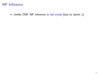
Download as PDF, PPTX

![Training CNP
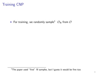
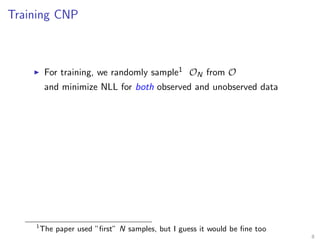
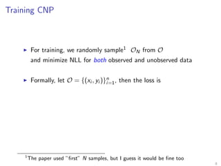
For training, we randomly sample1 ON from O
and minimize NLL for both observed and unobserved data
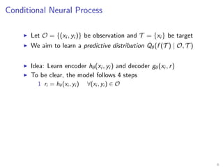
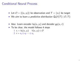
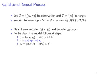
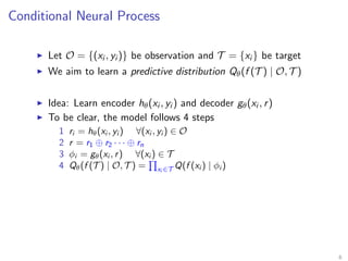
Formally, let O = {(xi , yi )}n
i=1, then the loss is
L(θ) = −Ef ∼P [EN [log Qθ(y1:n | ON, x1:n)]]
1
The paper used ”first” N samples, but I guess it would be fine too
8](https://image.slidesharecdn.com/180828neuralprocess-180828041301/85/Neural-Processes-25-320.jpg)
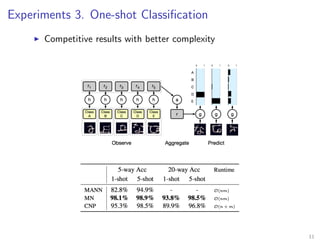
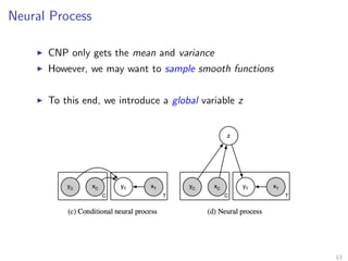
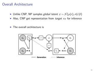
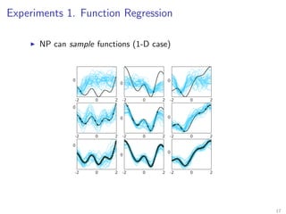
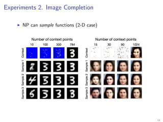
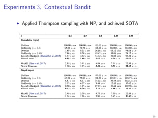
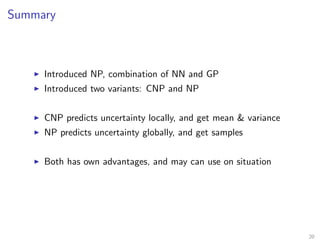

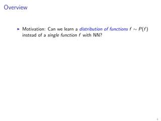
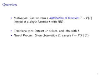
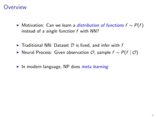
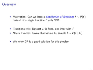
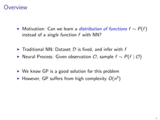
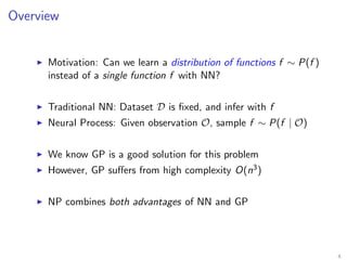
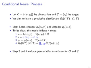
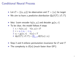
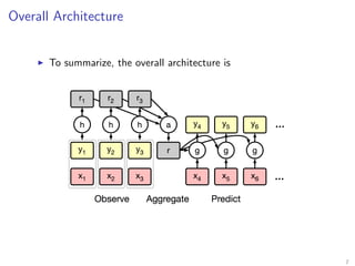
The document introduces Neural Processes (NP) and Conditional Neural Processes (CNP), which are models that aim to learn distributions of functions rather than single functions, improving upon traditional neural networks and Gaussian Processes. CNP focuses on predictive distributions given observations, while NP incorporates global latent variables for inference, allowing it to provide function samples and improve uncertainty estimates. The paper discusses architecture, complexity, training methods, and experiments demonstrating the efficacy of these models in tasks like regression and image completion.


![[DL輪読会]Conditional Neural Processes](https://cdn.slidesharecdn.com/ss_thumbnails/conditionalneuralprocesses-180727001730-thumbnail.jpg?width=640&height=640&fit=bounds)


![[DL輪読会]Wasserstein GAN/Towards Principled Methods for Training Generative Adv...](https://cdn.slidesharecdn.com/ss_thumbnails/wgan-1-170224021826-thumbnail.jpg?width=640&height=640&fit=bounds)


![[DL輪読会]近年のエネルギーベースモデルの進展](https://cdn.slidesharecdn.com/ss_thumbnails/energybasedmodel-200124020855-thumbnail.jpg?width=640&height=640&fit=bounds)


![[DL輪読会]World Models](https://cdn.slidesharecdn.com/ss_thumbnails/20180427-180427003856-thumbnail.jpg?width=640&height=640&fit=bounds)
![[DL輪読会]逆強化学習とGANs](https://cdn.slidesharecdn.com/ss_thumbnails/irlgans-171128063119-thumbnail.jpg?width=640&height=640&fit=bounds)


![[DL輪読会]Temporal DifferenceVariationalAuto-Encoder](https://cdn.slidesharecdn.com/ss_thumbnails/20181130new-190205051636-thumbnail.jpg?width=640&height=640&fit=bounds)

![[DL輪読会]Control as Inferenceと発展](https://cdn.slidesharecdn.com/ss_thumbnails/20191004-191204055019-thumbnail.jpg?width=640&height=640&fit=bounds)
![[DL輪読会]Inverse Constrained Reinforcement Learning](https://cdn.slidesharecdn.com/ss_thumbnails/20210709icrl-210709021811-thumbnail.jpg?width=640&height=640&fit=bounds)

![[DL輪読会]Convolutional Conditional Neural Processesと Neural Processes Familyの紹介](https://cdn.slidesharecdn.com/ss_thumbnails/20191220readingpaperconvcnp-191220034420-thumbnail.jpg?width=640&height=640&fit=bounds)
![[論文紹介] LSTM (LONG SHORT-TERM MEMORY)](https://cdn.slidesharecdn.com/ss_thumbnails/2018-181019021803-thumbnail.jpg?width=640&height=640&fit=bounds)