Download as PDF, PPTX


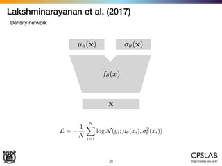
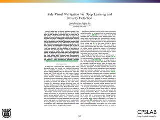
![Kendal & Gal (2017)
45
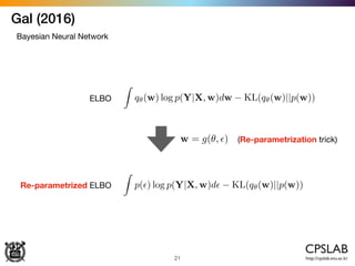
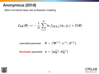
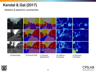
Aleatoric & epistemic uncertainties
ˆW ⇠ q(W)
x
ˆy ˆW(x) ˆ2
ˆW
(x)
[ˆy, ˆ2
] = f
ˆW
(x)
L =
1
N
NX
i=1
log N(yi; ˆy ˆW(x), ˆ2
ˆW
(x))](https://image.slidesharecdn.com/uncertainty-in-deep-learning-180106133211/85/Modeling-uncertainty-in-deep-learning-45-320.jpg)
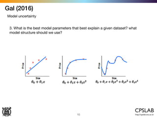
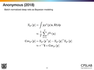
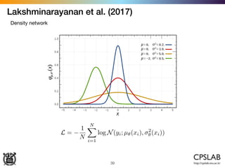
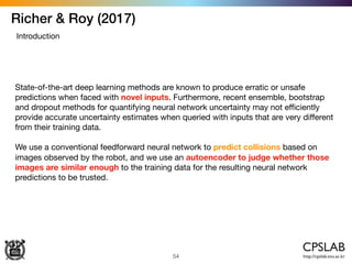
![Kendal & Gal (2017)
46
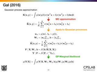
Heteroscedastic uncertainty as loss attenuation
ˆW ⇠ q(W)
x
ˆy ˆW(x) ˆ2
ˆW
(x)
[ˆy, ˆ2
] = f
ˆW
(x)](https://image.slidesharecdn.com/uncertainty-in-deep-learning-180106133211/85/Modeling-uncertainty-in-deep-learning-46-320.jpg)
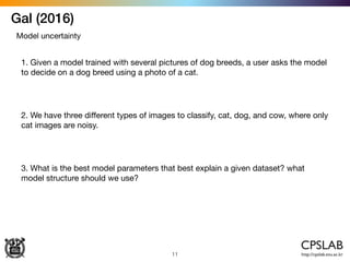
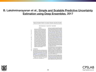
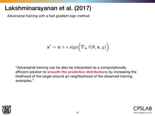
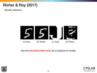
![Kendal & Gal (2017)
47
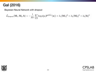
Aleatoric & epistemic uncertainties
ˆW ⇠ q(W)
x
ˆy ˆW(x) ˆ2
ˆW
(x)
[ˆy, ˆ2
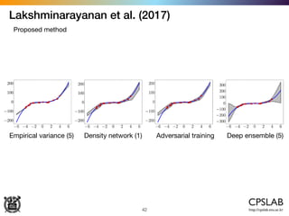
] = f
ˆW
(x)
Var(y) ⇡
1
T
TX
t=1
ˆy2
t
TX
t=1
ˆyt
!2
+
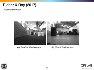
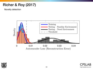
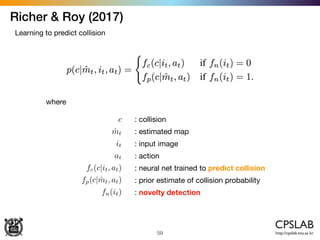
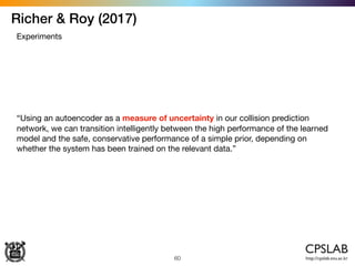
1
T
TX
t=1
ˆ2
t
Epistemic unct. Aleatoric unct,](https://image.slidesharecdn.com/uncertainty-in-deep-learning-180106133211/85/Modeling-uncertainty-in-deep-learning-47-320.jpg)
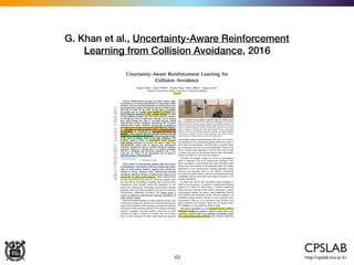
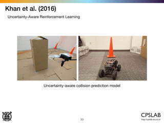
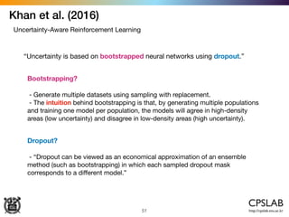
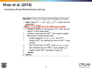
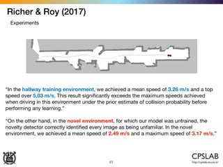
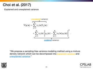


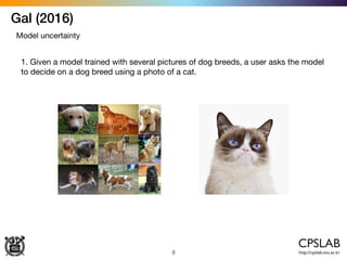
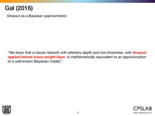
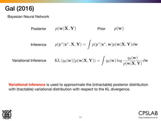
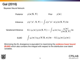
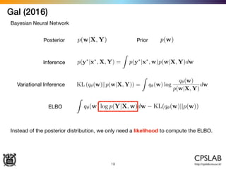
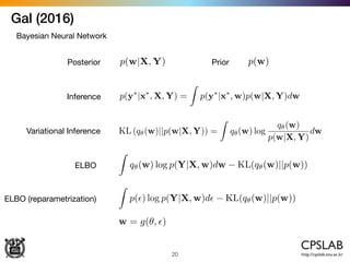
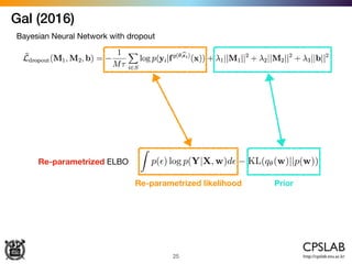
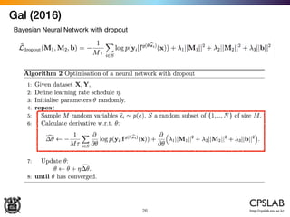
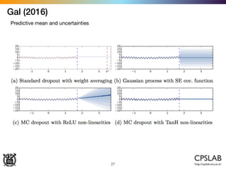
The document discusses the uncertainties in deep learning, highlighting examples of model uncertainty and the application of Bayesian neural networks for managing epistemic and aleatoric uncertainties. It covers various methodologies, including dropout as a Bayesian approximation, variational inference, and the use of mixture density networks to quantify uncertainties in predictive tasks. Additionally, it addresses approaches for safe reinforcement learning and the implications of these uncertainties in practical scenarios.