The document discusses the history and functioning of artificial neural networks (ANNs), drawing parallels between biological neural processes and computational models. It covers concepts like multilayer networks, back-propagation, and various applications, including handwriting and face recognition. Additionally, it provides examples of real-world datasets used to test and validate neural network predictions in supervised learning contexts.

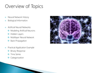
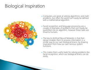
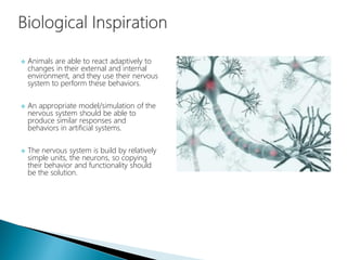
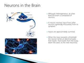
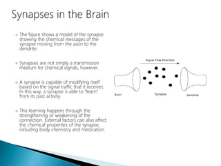
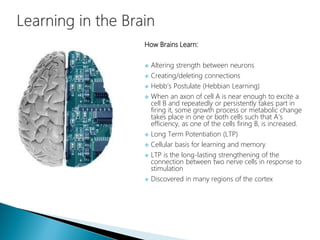
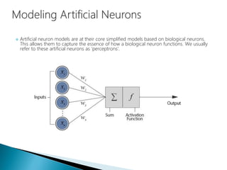
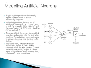
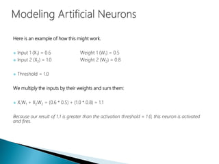
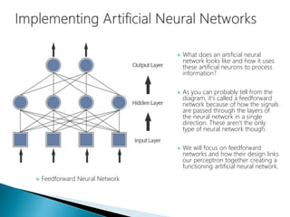
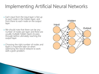
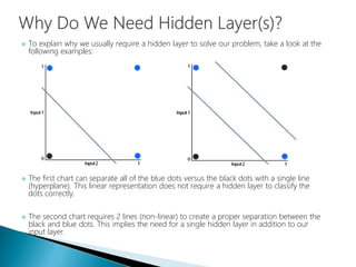
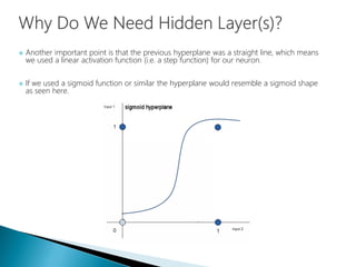
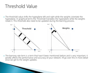
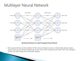
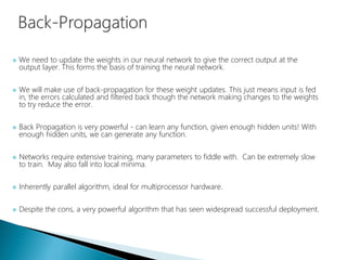
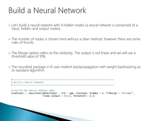
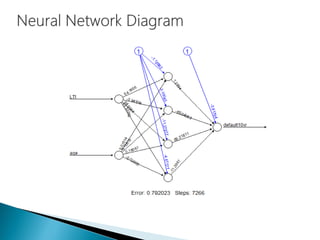
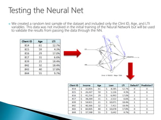
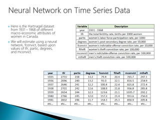
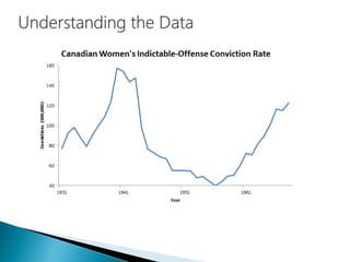
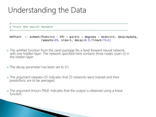
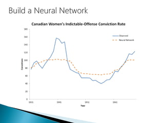
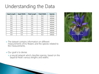
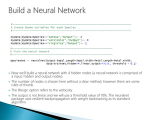
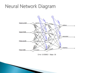
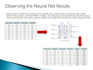
1. Presented by: Derek Kane

2.  Neural Network History
 Biological Information
 Artificial Neural Networks
 Modeling Artificial Neurons
 Hidden Layers
 Multilayer Neural Network
 Back-Propagation
 Practical Application Example
 Binary Response
 Time Series
 Categorization

3. History:
 History traces back to the 50’s but became popular in the 80’s with work by Rumelhart,
Hinton, and Mclelland
 A General Framework for Parallel Distributed Processing in Parallel Distributed Processing:
Explorations in the Microstructure of Cognition
 Hundreds of variants
 Less a model of the actual brain than a useful tool, but still some debate
Numerous applications:
 Handwriting, face, speech recognition
 Vehicles that drive themselves
 Models of reading, sentence production, dreaming

4.  Computers are great at solving algorithmic and math
problems, but often the world can't easily be defined
with a mathematical algorithm.
 Facial recognition and language processing are a
couple of examples of problems that can't easily be
quantified into an algorithm, however these tasks are
trivial to humans.
 The key to Artificial Neural Networks is that their
design enables them to process information in a
similar way to our own biological brains, by drawing
inspiration from how our own nervous system
functions.
 This makes them useful tools for solving problems like
facial recognition, which our biological brains can do
easily.

5.  Animals are able to react adaptively to
changes in their external and internal
environment, and they use their nervous
system to perform these behaviors.
 An appropriate model/simulation of the
nervous system should be able to
produce similar responses and
behaviors in artificial systems.
 The nervous system is build by relatively
simple units, the neurons, so copying
their behavior and functionality should
be the solution.

6.  Although heterogeneous, at a low
level the brain is composed of
neurons.
 A neuron receives input from other
neurons (generally thousands) from its
synapses.
 Inputs are approximately summed.
 When the input exceeds a threshold
the neuron sends an electrical spike
that travels that travels from the body,
down the axon, to the next neuron(s)

7.  The figure shows a model of the synapse
showing the chemical messages of the
synapse moving from the axon to the
dendrite.
 Synapses are not simply a transmission
medium for chemical signals, however.
 A synapse is capable of modifying itself
based on the signal traffic that it receives.
In this way, a synapse is able to “learn”
from its past activity.
 This learning happens through the
strengthening or weakening of the
connection. External factors can also affect
the chemical properties of the synapse,
including body chemistry and medication.

8. How Brains Learn:
 Altering strength between neurons
 Creating/deleting connections
 Hebb’s Postulate (Hebbian Learning)
 When an axon of cell A is near enough to excite a
cell B and repeatedly or persistently takes part in
firing it, some growth process or metabolic change
takes place in one or both cells such that A's
efficiency, as one of the cells firing B, is increased.
 Long Term Potentiation (LTP)
 Cellular basis for learning and memory
 LTP is the long-lasting strengthening of the
connection between two nerve cells in response to
stimulation
 Discovered in many regions of the cortex

10.  Artificial neuron models are at their core simplified models based on biological neurons.
This allows them to capture the essence of how a biological neuron functions. We usually
refer to these artificial neurons as 'perceptrons'.

11.  A typical perceptron will have many
inputs and these inputs are all
individually weighted.
 The perceptron weights can either
amplify or deamplify the original input
signal. For example, if the input is 1 and
the input's weight is 0.2 the input will be
decreased to 0.2.
 These weighted signals are then added
together and passed into the activation
function. The activation function is used
to convert the input into a more useful
output.
 There are many different types of
activation function but one of the
simplest would be step function. A step
function will typically output a 1 if the
input is higher than a certain threshold,
otherwise it's output will be 0.

12. Here is an example of how this might work.
 Input 1 (X1) = 0.6 Weight 1 (W1) = 0.5
 Input 2 (X2) = 1.0 Weight 2 (W2) = 0.8
 Threshold = 1.0
We multiply the inputs by their weights and sum them:
 X1W1 + X2W2 = (0.6 * 0.5) + (1.0 * 0.8) = 1.1
Because our result of 1.1 is greater than the activation threshold = 1.0, this neuron is activated
and fires.

13.  What does an artificial neural
network looks like and how it uses
these artificial neurons to process
information?
 As you can probably tell from the
diagram, it's called a feedforward
network because of how the signals
are passed through the layers of
the neural network in a single
direction. These aren't the only
type of neural network though.
 We will focus on feedforward
networks and how their design links
our perceptron together creating a
functioning artificial neural network.
 Feedforward Neural Network

14.  Each input from the input layer is fed up
to each node in the hidden layer, and
from there to each node on the output
layer.
 We should note that there can be any
number of nodes per layer and there are
usually multiple hidden layers to pass
through before ultimately reaching the
output layer.
 Choosing the right number of nodes and
layers is important later on when
optimizing the neural network to work
well a given problem.

15.  To explain why we usually require a hidden layer to solve our problem, take a look at the
following examples:
 The first chart can separate all of the blue dots versus the black dots with a single line
(hyperplane). This linear representation does not require a hidden layer to classify the
dots correctly.
 The second chart requires 2 lines (non-linear) to create a proper separation between the
black and blue dots. This implies the need for a single hidden layer in addition to our
input layer.

16.  Another important point is that the previous hyperplane was a straight line, which means
we used a linear activation function (i.e. a step function) for our neuron.
 If we used a sigmoid function or similar the hyperplane would resemble a sigmoid shape
as seen here.

17.  The threshold value shifts the hyperplane left and right while the weights orientate the
hyperplane. In graphical terms the Threshold translates the hyperplane while the weights
rotate it. This threshold also need to be updated during the learning process.
 The learning rate term is a term that hasn't been mentioned before and is very important, it
greatly affects the performance and accuracy of your network. I’ll go over this in more detail
once we get to the weight updates.
WeightsThreshold

18.  The square blocks at the bottom of this neural network are our thresholds (bias) values.
These neurons are then hooked up to the rest of the network and have their own weights
(these are technically the threshold values).

19.  We need to update the weights in our neural network to give the correct output at the
output layer. This forms the basis of training the neural network.
 We will make use of back-propagation for these weight updates. This just means input is fed
in, the errors calculated and filtered back though the network making changes to the weights
to try reduce the error.
 Back Propagation is very powerful - can learn any function, given enough hidden units! With
enough hidden units, we can generate any function.
 Networks require extensive training, many parameters to fiddle with. Can be extremely slow
to train. May also fall into local minima.
 Inherently parallel algorithm, ideal for multiprocessor hardware.
 Despite the cons, a very powerful algorithm that has seen widespread successful deployment.

20.  The weight changes are calculated by using the gradient descent method. This means we
follow the steepest path on the error function to try and minimize it.
 All we’re doing is just taking the error at the output neurons (Desired value – actual value)
and multiplying it by the gradient of the sigmoid function. If the difference is positive we
need to move up the gradient of the activation function and if its negative we need to move
down the gradient of the activation function.

21.  This is the formula to calculate the basic error gradient for each output neuron k:
 There is a difference between the error gradients at the output and hidden layers.
 The hidden layer’s error gradient is based on the output layer’s error gradient (back
propagation) so for the hidden layer the error gradient for each hidden neuron is the
gradient of the activation function multiplied by the weighted sum of the errors at the output
layer originating from that neuron.

22.  The final step in the algorithm is to update the weights, this occurs as follows:
 The alpha value you see above is the learning rate, this is usually a value between 0 and 1. It
affects how large the weight adjustments are and so also affects the learning speed of the
network. This value need to be careful selected to provide the best results, too low and it will
take a long time to learn, too high and the adjustments might be too large and the accuracy
will suffer as the network will constantly jump over a better solution and generally get stuck at
some sub-optimal accuracy.

23.  The Back-Propagation Algorithm learns during a training epoch, you will probably go
through several epochs before the network has sufficiently learned to handle all the data
you’ve provided it and the end result is satisfactory.
A training epoch is described below:
For each input entry in the training data set:
 feed input data in (feed forward)
 check output against desired value and feed back error (back-propagate)
Where back-propagation consists of:
 calculate error gradients
 update weights

25. These are some commonly used stopping conditions used for neural networks:
 Desired accuracy
 Desired mean square error
 Elapsed epochs

26.  We just discussed a form of supervised learning
 A “teacher” tells the network what the correct output is based on the input until the
network learns the target concept.
 We can also train networks where there is no teacher. This is called unsupervised learning.
The network learns a prototype based on the distribution of patterns in the training data.
Such networks allow us to:
 Discover underlying structure of the data
 Encode or compress the data
 Transform the data
 This presentation will focus on the supervised learning form consisting of a feed forward ANN
with back propagation. However, it is important to understand that, like the human brain,
there are many complexities within neural networks and different architectures that can be
employed depending on the modeling task at hand.

28.  The dataset contains information on different banking clients who received a loan at least 10
years ago.
 The variables income (yearly), age, loan (size in euros) and LTI (the loan to yearly income
ratio) are available.
 Our goal is to devise:
 a neural network which predicts, based on the input variables LTI and age,
 whether or not a default will occur within 10 years.

29.  Let’s build a neural network with 4 hidden nodes (a neural network is comprised of a
input, hidden and output nodes).
 The number of nodes is chosen here without a clear method, however there are some
rules of thumb.
 The lifesign option refers to the verbosity. The output is not linear and we will use a
threshold value of 10%.
 The neuralnet package in R uses resilient backpropagation with weight backtracking as
its standard algorithm.

31.  We created a random test sample of the dataset and included only the Clint ID, Age, and LTI
variables. This data was not involved in the initial training of the Neural Network but will be used
to validate the results from passing the data through the NN.

33.  Here is the Hartnagel dataset
from 1931 – 1968 of different
macro-economic attributes of
women in Canada.
 We will estimate using a neural
network, fconvict, based upon
values of tfr, partic, degrees,
and mconvict.

35.  The avNNet function from the caret package fits a feed-forward neural network
with one hidden layer. The network specified here contains three nodes (size=3) in
the hidden layer.
 The decay parameter has been set to 0.1.
 The argument repeats=25 indicates that 25 networks were trained and their
predictions are to be averaged.
 The argument linout=TRUE indicates that the output is obtained using a linear
function.

38. Setosa Virginica Versicolor

39.  The dataset contains information on different
measurements of Iris flowers and the species related to
the measurements.
 Our goal is to devise:
 a neural network which classifies species, based on the
Sepal & Petal’s various lengths and widths.

40.  Now we’ll build a neural network with 4 hidden nodes (a neural network is comprised of
a input, hidden and output nodes).
 The number of nodes is chosen here without a clear method, however there are some
rules of thumb.
 The lifesign option refers to the verbosity.
 The output is not linear and we will use a threshold value of 10%. The neuralnet
package uses resilient backpropagation with weight backtracking as its standard
algorithm.

42.  We created a random test sample of the dataset and included only the Sepal Length, Sepal
Width, Petal Length, and Petal Width variables. This data was not involved in the initial training of
the Neural Network but will be used to validate the results from passing the data through the NN.

43.  Reside in Wayne, Illinois
 Active Semi-Professional Classical Musician
(Bassoon).
 Married my wife on 10/10/10 and been
together for 10 years.
 Pet Yorkshire Terrier / Toy Poodle named
Brunzie.
 Pet Maine Coons’ named Maximus Power and
Nemesis Gul du Cat.
 Enjoy Cooking, Hiking, Cycling, Kayaking, and
Astronomy.
 Self proclaimed Data Nerd and Technology
Lover.