Download as PDF, PPTX


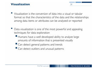


The document outlines data exploration techniques, emphasizing the importance of understanding data characteristics before analysis. It highlights exploratory data analysis (EDA) as a key practice for uncovering insights without preconceived hypotheses, focusing on methods such as summary statistics, visualization techniques, and the significance of recognizing patterns. Various visualization methods like bar plots, histograms, box plots, and scatter plots are discussed to aid in analyzing data relationships and distributions.