Downloaded 277 times


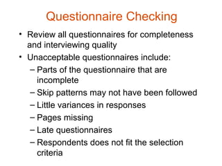
![Data Coding
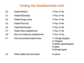
• Assigning a code [number] to each possible
response to each question [variable]
– Structured questionnaires [pre-coded]
– Unstructured questions [post-coding]
• Category codes should be mutually exclusive
and collectively exhaustive.
• Category codes should be assigned for critical
issues even if no one mentions them.](https://image.slidesharecdn.com/lecture8fundamentalsofdataanalysis-121005005439-phpapp02/85/Fundamentals-of-data-analysis-10-320.jpg)

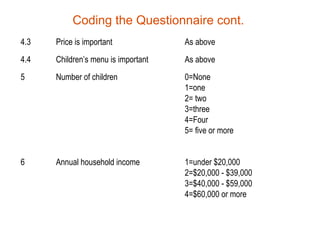
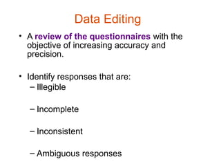
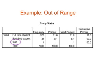
![Data Cleaning
• Consistency check
– Out of range [see study status]
– Logically inconsistent
[e.g., does not own the product but is a heavy user]
– Extreme values
[indiscriminatingly responding the same way on all attributes]](https://image.slidesharecdn.com/lecture8fundamentalsofdataanalysis-121005005439-phpapp02/85/Fundamentals-of-data-analysis-17-320.jpg)
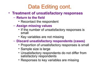
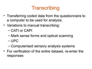
![Data Cleaning cont.
• Treatment of missing responses
– Substitute a neutral value [substitute the ‘mean’
response of the variable]
– Substitute an imputed response [use the
respondent’s pattern of responses to other
questions]
– Casewise deletion [respondents with any missing
values are discarded from the analysis]
– Pairwise deletion [use only cases or respondents
with complete responses for each calculation]](https://image.slidesharecdn.com/lecture8fundamentalsofdataanalysis-121005005439-phpapp02/85/Fundamentals-of-data-analysis-19-320.jpg)
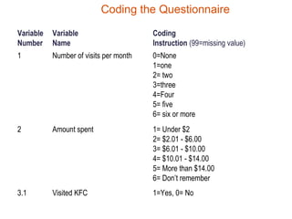
![Statistically Adjusting the Data
• Weighting
– Each case is assigned a weight to reflect its
importance relative to other cases, often used to
make the sample more representative of a target
population
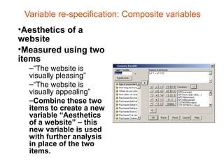
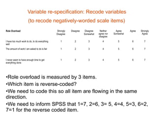
• Variable re-specification
– Transformation of data to create new variables or
modify existing variables to better suit the
research objectives by summing several variables,
log transformations, dummy variables [see next
slide]
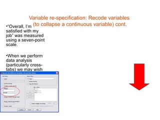
• Scale transformation
– Manipulation of scale values to ensure
comparability with other scales or otherwise make
the data suitable for analysis [when data is not
normally distributed].](https://image.slidesharecdn.com/lecture8fundamentalsofdataanalysis-121005005439-phpapp02/85/Fundamentals-of-data-analysis-20-320.jpg)
![Strategy for Data Analysis
• Determine the type of data which is available
[nominal, ordinal, interval, ratio]
• Decide what needs to be discussed in order to tell
‘the story’
• Choose techniques to best get information on
specific parts of what has to be discussed
• Run the results
• Determine what the results mean, what patterns
can be seen, what kind of statistical decisions
should be made
• Write about the results to explain what is going on
to someone who does not like numbers and has
never heard of statistics](https://image.slidesharecdn.com/lecture8fundamentalsofdataanalysis-121005005439-phpapp02/85/Fundamentals-of-data-analysis-24-320.jpg)
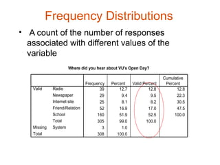
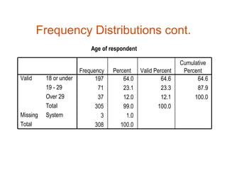
![Overview of Techniques
• Descriptive Statistics
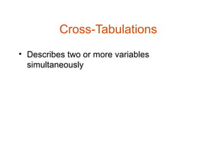
– Frequency distribution and cross
tabulations
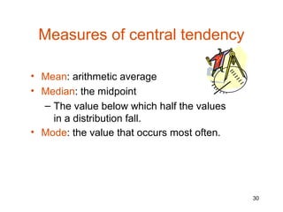
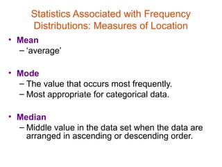
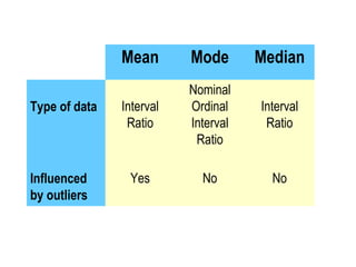
– Measures of central tendency [mean,
median, mode]
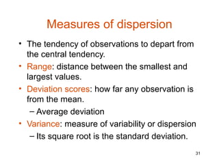
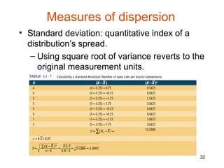
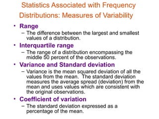
– Measures of dispersion [range,
interquartile range, standard deviation]
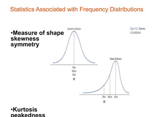
– Shape [skewness, kurtosis]
• Inferential Statistics
– Parametric tests [Z or t test, paired t
test]
– Non-parametric tests [Chi-square]](https://image.slidesharecdn.com/lecture8fundamentalsofdataanalysis-121005005439-phpapp02/85/Fundamentals-of-data-analysis-25-320.jpg)
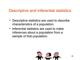
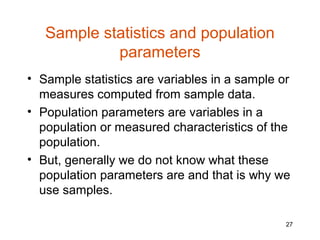
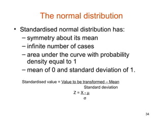
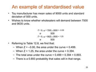
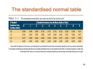
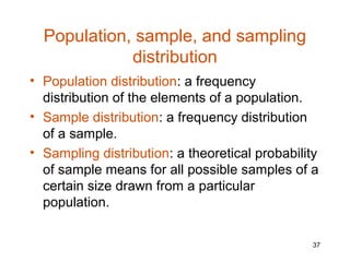
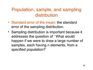
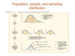
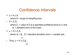
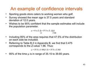


The document provides an overview of univariate statistical analysis and inferential statistics, including key concepts like population and sample distributions, measures of central tendency and dispersion, the normal distribution, sampling distributions, confidence intervals, and how these statistical techniques are used to make inferences about populations based on samples. It also discusses important steps in the data analysis process like data preparation, selecting appropriate analysis strategies and techniques based on the research objectives and data types.


![Big Data [sorry] & Data Science: What Does a Data Scientist Do?](https://cdn.slidesharecdn.com/ss_thumbnails/dslatcloudmsevent20130125-130126065651-phpapp01-thumbnail.jpg?width=640&height=640&fit=bounds)


