- Centrifugal pumps use impellers to impart velocity and pressure to fluids. Impellers can have single or multiple stages. - Affinity laws describe how flow rate, head, speed, and power relate as variables change. Centrifugal pump performance can be predicted using these scaling relationships. - Specific speed is used to classify pumps based on geometric similarity. Euler's and Bernoulli's equations relate velocities, pressures, and heads in centrifugal pumps. - Stepanoff's method uses empirical coefficients to design centrifugal pumps based on design parameters like flow rate, head, speed, and impeller dimensions. Blade thickness affects internal velocities.

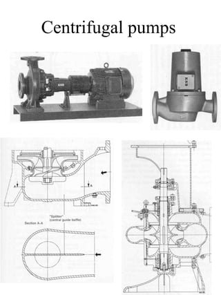
1. Centrifugal pumps

3. Impellers

4. Multistage impellers

5. Cross section of high speed
water injection pump
Source: www.framo.no

6. Water injection unit
4 MW
Source: www.framo.no

7. Specific speed that is used to
classify pumps
nq is the specific speed for a unit machine that
is geometric similar to a machine with the head
Hq = 1 m and flow rate Q = 1 m3
/s
43q
H
Q
nn ⋅=
qs n55,51n ⋅=

9. Affinity laws
2
1
2
1
n
n
Q
Q
=
2
2
1
2
2
1
2
1
n
n
u
u
H
H






=





=
3
2
1
2
1
n
n
P
P






=
Assumptions:
Geometrical similarity
Velocity triangles are the same

10. Exercise
sm1,11
1000
1100
Q
n
n
Q 3
1
1
2
2 =⋅=⋅=
m121100
1000
1100
H
n
n
H
2
1
2
1
2
2 =⋅





=⋅





=
kW164123
1000
1100
P
n
n
P
3
1
3
1
2
2 =⋅





=⋅





=
• Find the flow rate, head and power
for a centrifugal pump that has
increased its speed
• Given data:
ηh = 80 % P1 = 123 kW
n1 = 1000 rpm H1 = 100
m
n2 = 1100 rpm Q1 = 1 m3
/s

11. Exercise
• Find the flow rate, head and power
for a centrifugal pump impeller that
has reduced its diameter
• Given data:
ηh = 80 % P1 = 123 kW
D1 = 0,5 m H1 = 100 m
D2 = 0,45 m Q1 = 1 m3
/s
sm9,01
5,0
45,0
Q
D
D
Q
n
n
D
D
cBD
cBD
Q
Q
3
1
1
2
2
2
1
2
1
2m22
1m11
2
1
=⋅=⋅=
⇓
==
⋅⋅⋅Π
⋅⋅⋅Π
=
m81100
5,0
45,0
H
D
D
H
2
1
2
1
2
2 =⋅





=⋅





=
kW90123
5,0
45,0
P
D
D
P
3
1
3
1
2
2 =⋅





=⋅





=

12. Velocity triangles

14. Slip angle
Reduced cu2
Slip angle
Slip
Best efficiency point
Friction loss
Impulse loss

15. Power
ω⋅= MP
Where:
M = torque [Nm]
ω = angular velocity [rad/s]
( )
( )
t
1u12u2
111222
HgQ
cucuQ
coscrcoscrQP
⋅⋅⋅ρ=
ω⋅⋅−⋅⋅⋅ρ=
ω⋅α⋅⋅−α⋅⋅⋅⋅ρ=

16. g
cucu
H 1u12u2
t
⋅−⋅
=
In order to get a better understanding of
the different velocities that represent the
head we rewrite the Euler’s pump
equation
1u1
2
1
2
1111
2
1
2
1
2
1 cu2uccoscu2ucw ⋅⋅−+=α⋅⋅⋅−+=
2u2
2
2
2
2222
2
2
2
2
2
2 cu2uccoscu2ucw ⋅⋅−+=α⋅⋅⋅−+=
g2
ww
g2
cc
g2
uu
H
2
1
2
2
2
1
2
2
2
1
2
2
t
⋅
−
−
⋅
−
+
⋅
−
=

17. Euler’s pump equation
g
cucu
H 1u12u2
t
⋅−⋅
=
g2
ww
g2
cc
g2
uu
H
2
1
2
2
2
1
2
2
2
1
2
2
t
⋅
−
−
⋅
−
+
⋅
−
=
=
⋅
−
g2
uu 2
1
2
2 Pressure head due to change of
peripheral velocity
=
⋅
−
g2
cc 2
1
2
2
=
⋅
−
g2
ww 2
1
2
2
Pressure head due to change of
absolute velocity
Pressure head due to change of
relative velocity

18. Rothalpy
Using the Bernoulli’s equation upstream and
downstream a pump one can express the
theoretical head:
1
2
2
2
t z
g2
c
g
p
z
g2
c
g
p
H 





+
⋅
+
⋅ρ
−





+
⋅
+
⋅ρ
=
g2
ww
g2
cc
g2
uu
H
2
1
2
2
2
1
2
2
2
1
2
2
t
⋅
−
−
⋅
−
+
⋅
−
=
The theoretical head can also be expressed as:
Setting these two expression for the theoretical
head together we can rewrite the equation:
g2
u
g2
w
g
p
g2
u
g2
w
g
p 2
1
2
11
2
2
2
22
⋅
−
⋅
+
⋅ρ
=
⋅
−
⋅
+
⋅ρ

19. Rothalpy
The rothalpy can be written as:
( )
ttancons
g2
r
g2
w
g
p
I
22
=
⋅
⋅ω
−
⋅
+
⋅ρ
=
This equation is called the
Bernoulli’s equation for
incompressible flow in a rotating
coordinate system, or the rothalpy
equation.

20. Stepanoff
We will show how a centrifugal pump is designed
using Stepanoff’s empirical coefficients.
Example: H = 100 m
Q = 0,5 m3
/s
n = 1000 rpm
β2 = 22,5 o

21. 4,22
100
5,0
1000
H
Q
nn 4343q =⋅=⋅=
1153n55,51n qs =⋅=
Specific speed:
This is a radial pump

22. 0,1Ku =
sm3,44Hg2Ku
Hg2
u
K u2
2
u =⋅⋅⋅=⇒
⋅⋅
=
srad7,104
60
n2
=
⋅Π⋅
=ω
m85,0
2u
D
2
D
u 2
2
2
2 =
ω
⋅
=⇒⋅ω=
We choose: m17,0D5,0D 1hub =⋅=

23. 11,0K 2m =
sm87,4Hg2Kc
Hg2
c
K 2m2m
2m
2m =⋅⋅⋅=⇒
⋅⋅
=
m038,0
cD
Q
d
dD
Q
A
Q
c
2m2
2
22
2m
=
⋅⋅Π
=
⇓
⋅⋅Π
==
u2
c2
w2
cu2
cm2

24. Thickness of the blade
Until now, we have not considered the thickness
of the blade. The meridonial velocity will
change because of this thickness.
( )
( )
m039,0
cszD
Q
d
dszD
Q
A
Q
c
2mu2
2
2u2
2m
=
⋅⋅−⋅Π
=
⇓
⋅⋅−⋅Π
==
We choose: s2 = 0,005 m
z = 5
m013,0
5,22sin
005,0
sin
s
s o
2
2
u ==
β
=

25. 145,0K 1m =
sm4,6Hg2Kc
Hg2
c
K 1m1m
1m
1m =⋅⋅⋅=⇒
⋅⋅
=
u1
w1
c1= cm1

26. 405,0
D
D
2
1
=
m34,0D405,0D405,0
D
D
21
2
1
=⋅=⇒=
m09,0
cD
Q
d
dD
Q
A
Q
c
1mm1
1
1m11
1m =
⋅⋅Π
=⇒
⋅⋅Π
==
We choose:
Dhub
m17,0D5,0D 1hub =⋅=
m27,0
2
DD
D
2
hub
2
1
m1 =
+
=
Without thickness

27. Thickness of the blade at
the inlet
m015,0
8,19sin
005,0
sin
s
s o
1
1
1u ==
β
=
u1
w1
Cm1=6,4 m/s
sm8,17
2
34,0
7,104
2
D
u 1
1 =⋅=⋅ω=
β1
o
1
1m
1 8,19
8,17
4,6
tana
u
c
tana =





=





=β
( )
m10,0
cszD
Q
d
1m1um1
1 =
⋅⋅−⋅Π
=

28. m153
81,996,0
5,323,44
g
cucu
H
h
1u12u2
=
⋅
⋅
=
⋅η
⋅−⋅
=
u2=44,3 m/s
c2
w2
cm2=4,87m/s
β2=22,5o
cu2
sm5,32
tan
c
uc
cu
c
tan
2
2m
22u
2u2
2m
2 =
β
−=⇒
−
=β

29. u2=44,3 m/s
c2
w2
cm2=4,87m/s
cu2
sm3,21
3,44
81,996,0100
u
gH
c
g
cu
H
2
h
2u
h
2u2
=
⋅⋅
=
⋅η⋅
=⇒
⋅η
⋅
=
o
2u2
2m
2 9,11
3,213,44
87,4
tana
cu
c
tana' =
−
=
−
=β
ooo
2slipslip 6,109,115,22' =−=β−β=β