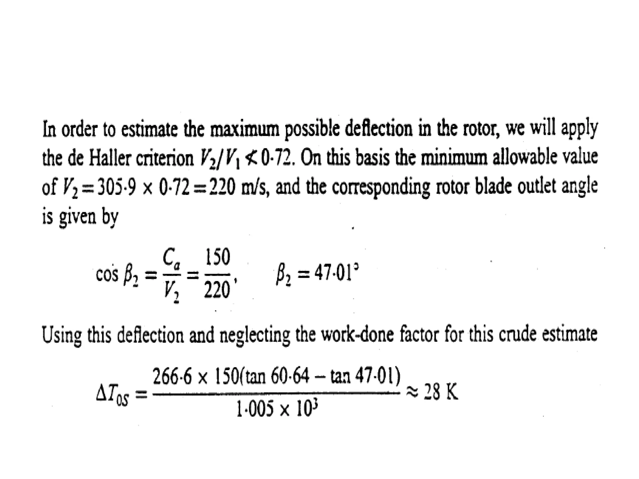
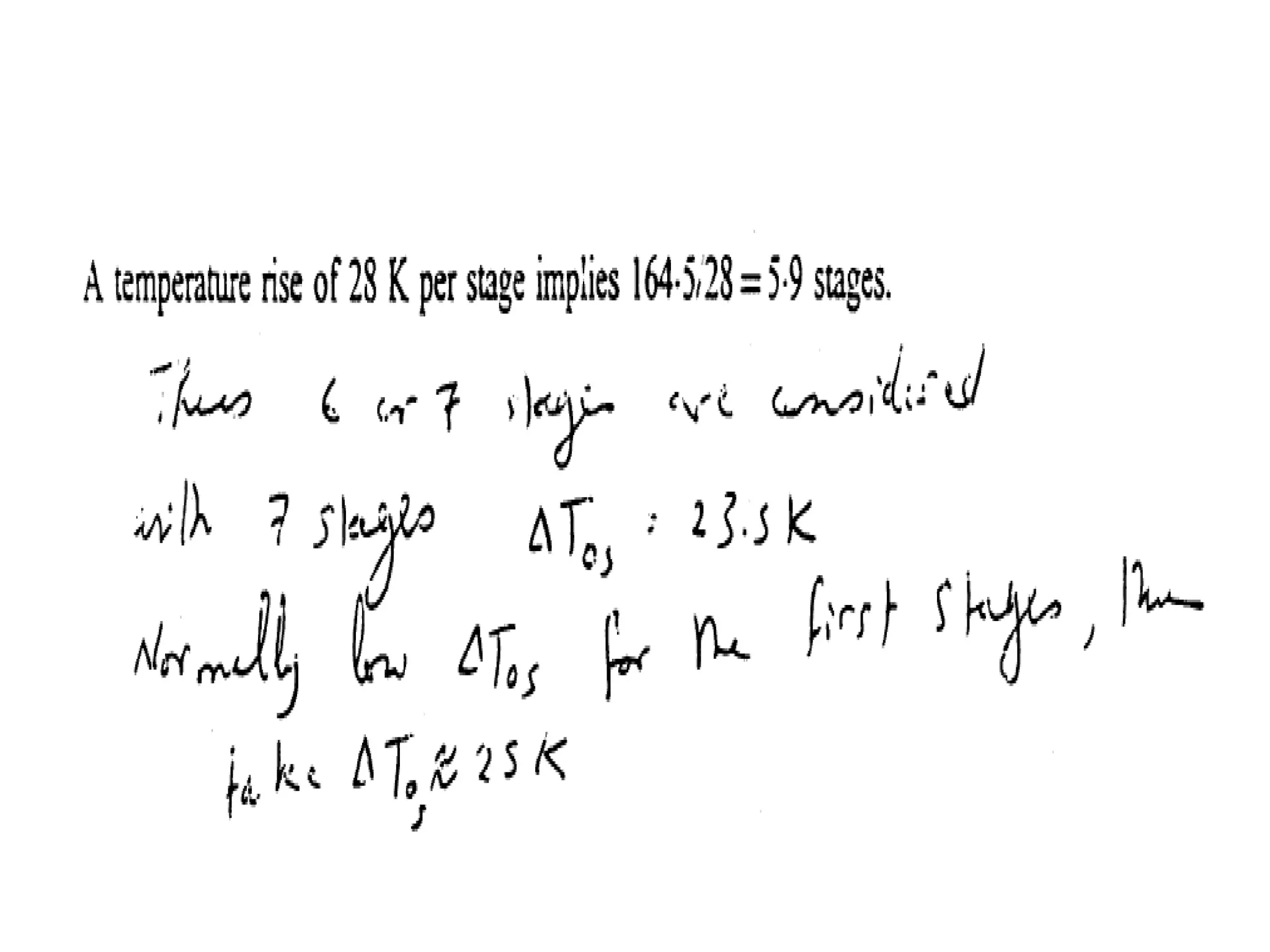
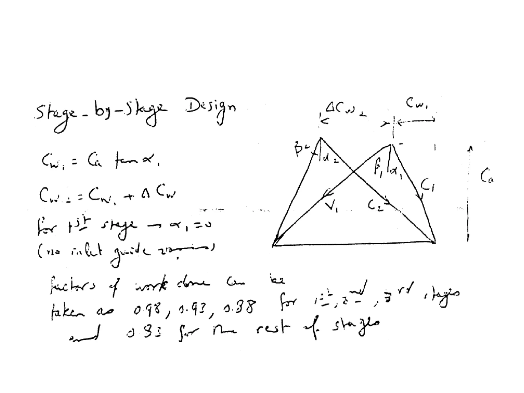
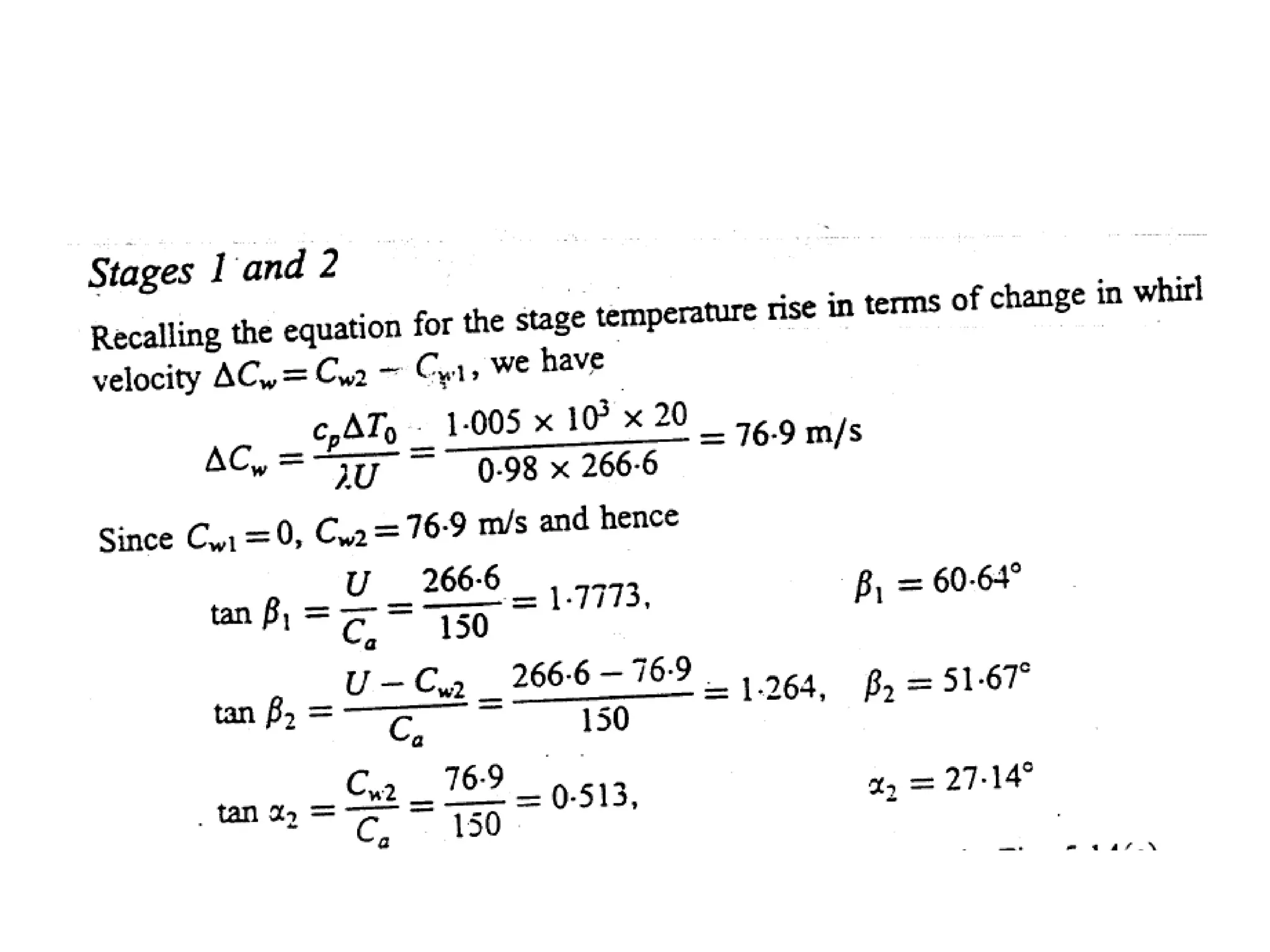
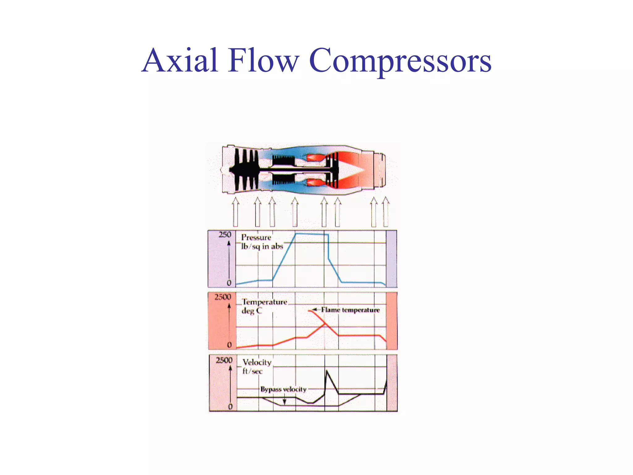
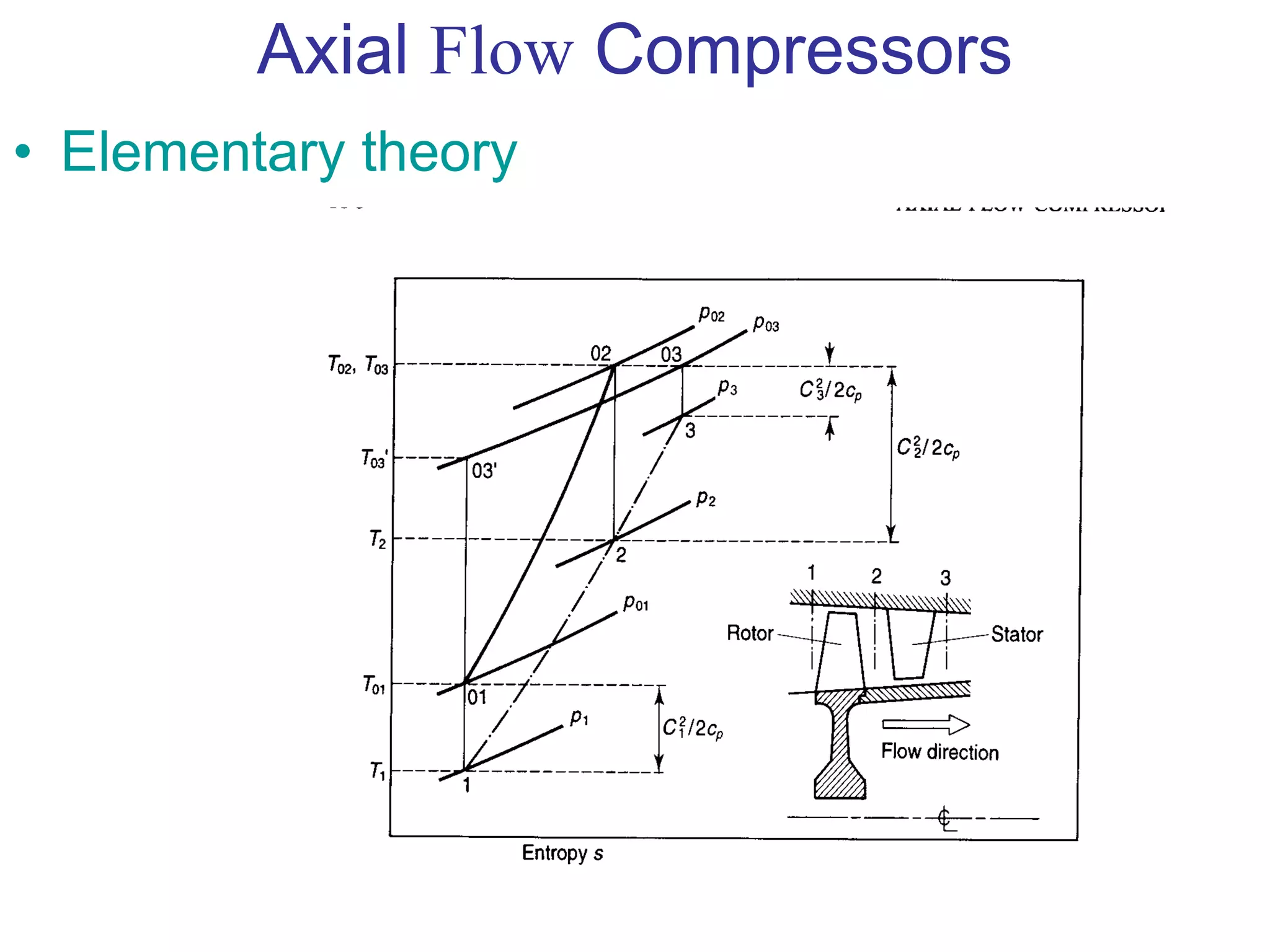
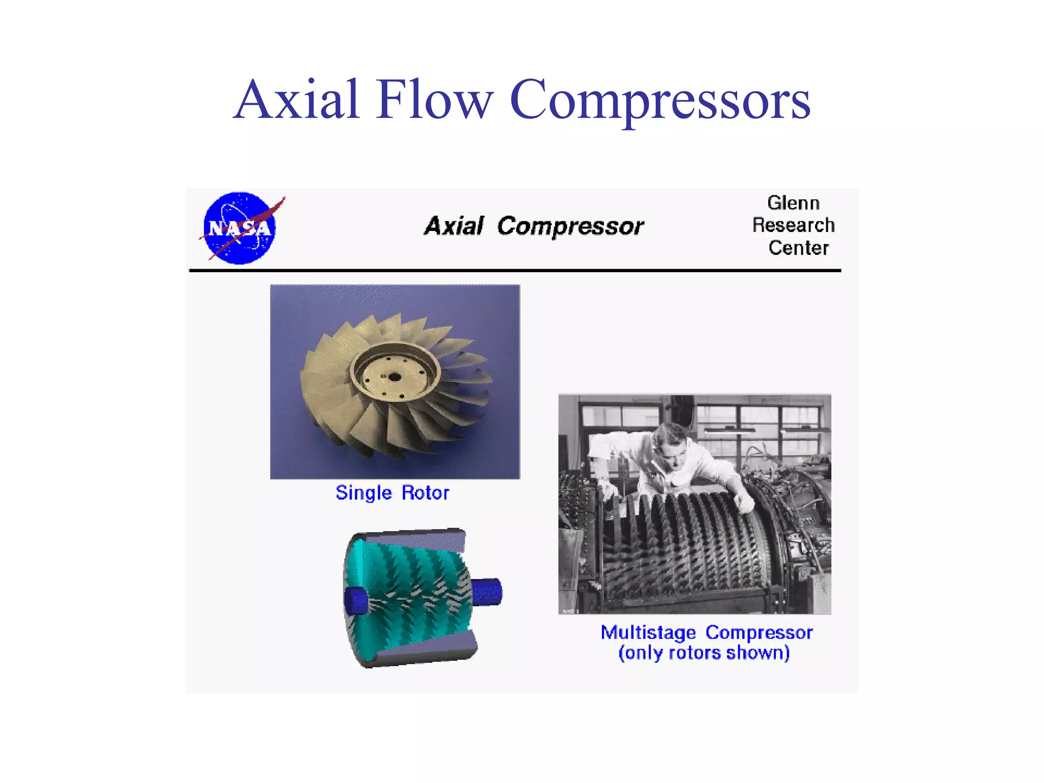
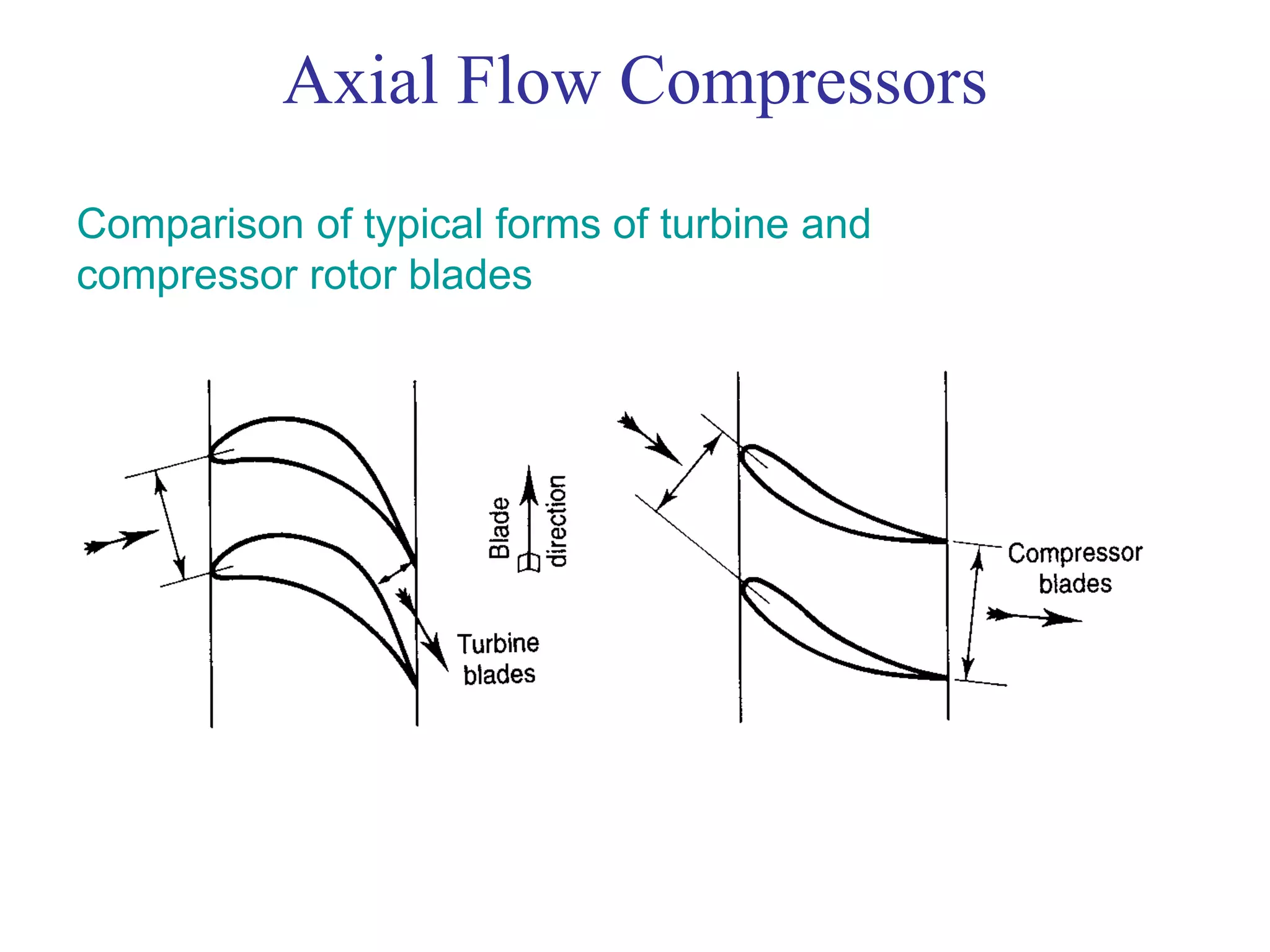
The document discusses axial flow compressors. It begins with an overview that axial flow compressors have multiple stages, each with a row of rotor blades followed by a row of stator blades. The fluid is accelerated by the rotor blades and decelerated in the stator, converting kinetic to static pressure energy. Due to small pressure increases per stage, axial compressors require many stages. The document then provides details on the elementary theory, velocity triangles, degree of reaction, and three dimensional flow effects in axial compressors. It concludes with discussing the design process which includes choosing operating parameters, determining number of stages, calculating air angles, and testing.

1. Axial Flow Compressors

2. Axial Flow Compressors
• Elementary theory

3. Axial Flow Compressors

4. Axial Flow Compressors
Comparison of typical forms of turbine and
compressor rotor blades

5. Axial Flow Compressors
Axial Flow Compressors
Stage= S+R
S: stator (stationary blade)
R: rotor (rotating blade)
First row of the stationary blades is called guide vanes
** Basic operation
*Axial flow compressors:
1) series of stages
2) each stage has a row of rotor blades followed
by a row of stator blades.
3) fluid is accelerated by rotor blades.

6. Axial Flow Compressors
In stator, fluid is then decelerated causing change in the
kinetic energy to static pressure.
Due to adverse pressure gradient, the pressure rise for
each stage is small. Therefore, it is known that a single
turbine stage can drive a large number of compressor
stages.
Inlet guide vanes are used to guide the flow into the first
stage.
Elementary Theory:
Assume mid plane is constant r1=r2, u1=u2
assume Ca=const, in the direction of u.
12 www CCC 
, in the direction of u.12 www CCC 

7. Axial Flow Compressors
Inside the rotor, all power is consumed.
Stator only changes K.E.P static, To2=To3
Increase in stagnation pressure is done in the rotor.
Stagnation pressure drops due to friction loss in the stator:
C1: velocity of air approaching the rotor.
1 : angle of approach of rotor.
u: blade speed.
V1: the velocity relative t the rotor at inlet at an
angle 1 from the axial direction.
V2: relative velocity at exit rotor at angle 2
determined from the rotor blade outlet angle.
2: angle of exit of rotor.
Ca: axial velocity.

8. Axial Flow Compressors
Two dimensional analysis:
Only axial ( Ca) and tangential (Cw). no radial component
13
13
22
222
a
2
11
Calso
stagesimilaratogoair toprepareto
Cgetu triangle&V
cosVontainedbeV
Cassuming
exit.atbladetangnt to
2
21
C
normally
then
Ccanthis
CC
V
VuC
a
aa











)( 12
.
oop TTcmW 

9. Axial Flow Compressors

10. Axial Flow Compressors
)tan-(tan)tan-(tan 2112  
21 aaa CCC 
(a)tantan/,tantanu/Ca 2211   aCu
from velocity triangles
assuming
the power input to stage )(mW 12
'
ww CCu 
rotors.theofexitandinletatcomponentsltangentiaare21 ww andCC
where
or in terms of the axial velocity
From equation (a)
)tan-(tanmuCW 12a 

11. Axial Flow Compressors
Energy balance
pao
aoooopop
cuCT
uCTTcTTcTc
/)tan(tan
)tan(tan)()(
21
21
5
12135




pressure ratio at a stage
3 5
1 1
1
1
s
1
2
1 where, isentropic efficiency
Ex.
u 180 m/s, 43.9 , 0.85, 0.8,
150 / , 13.5, 288, 1.183 ,
higher due to centrifugal action
o s o
s
o o
o
s
a o s centrifugal
p T
p stage
p T
C m s T R R



  

 
    
  
   
    

12. Axial Flow Compressors

Degree of reaction
enthalpy rise in rotor
enthalpy rise in the stage
r
s
hstatic
static h

  

is the ratio of static enthalpy in rotor to static enthalpy
rise in stage
For incompressible isentropic flow Tds=dh-vdp
dh=vdp=dp/ Tds=0
h=p/ ( constant )
Thus enthalpy rise could be replaced by static pressure rise
( in the definition of )
1o but generally choose =0.5 at mid-plane of
the stage.

13. Axial Flow Compressors
=0: all pressure rise only in stator
=1: all pressure rise in only in rotor
=0.5: half of pressure rise only in rotor and half is in
stator. ( recommend design)
3 1 aAssume C ,and C . ( for simplicity)C const 
5
1 21 (tan tan ) / 2
o stagnation stage s
a
T T T T
C u 

    
   
uCa /,tan1   
1 2tan (tan tan )/ 2   

14. Axial Flow Compressors
special condition
=0 ( impulse type rotor)
from equation 3
1 2(tan tan )/ 2aC u   
1=-2 , velocities skewed left, h1=h2, T1=T2
=1.0 (impulse type stator from equation 1)
=1-Ca(tan1+tan2)/2u, 2=1
velocities skewed right, C1=C2, h2=h3T2=T3
1 2
1
(tan tan )
2 2

    
2 1
2 1
2 1 1 2
3 1
; symmetric angles
V , ;
P P
c V c
P P
 

   

=0.5
from 2

15. Axial Flow Compressors
Three dimensional flow
2-D
1. the effects due to radial movement of the fluid are ignored.
2. It is justified for hub-trip ratio>0.8
3. This occurs at later stages of compressor.
3-D are valid due to
1. due to difference in hub-trip ratio from inlet stages to
later-stages, the annulus will have a substantial taper.
Thus radial velocity occurs.
2. due to whirl component, pressure increase with
radius.

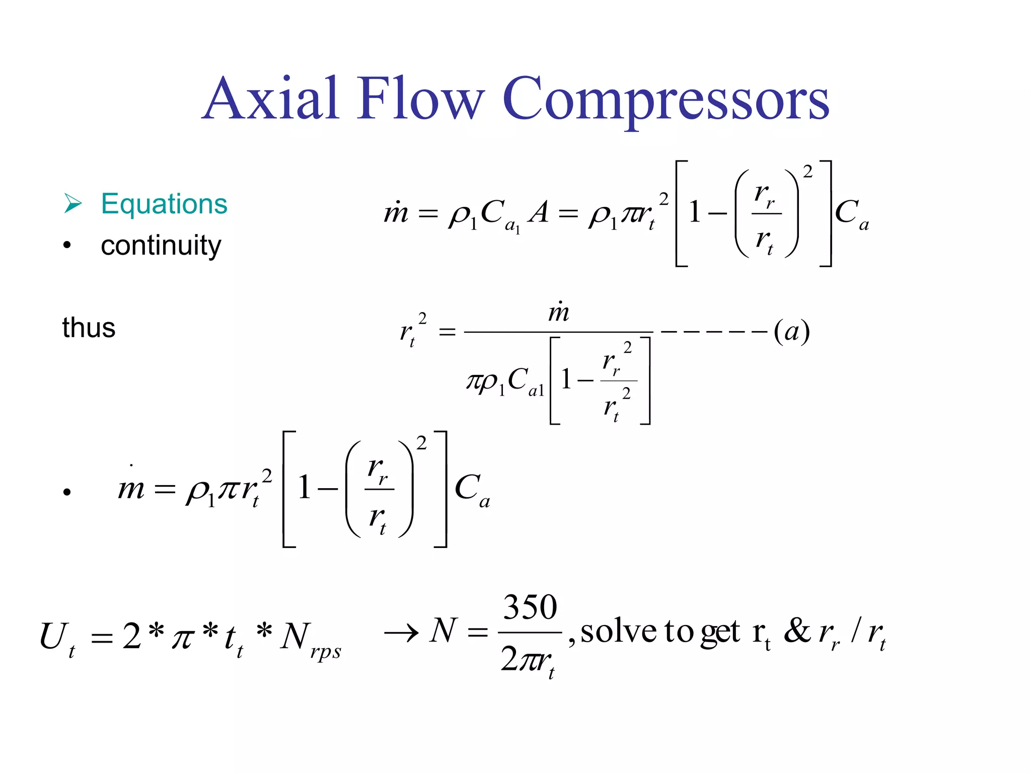
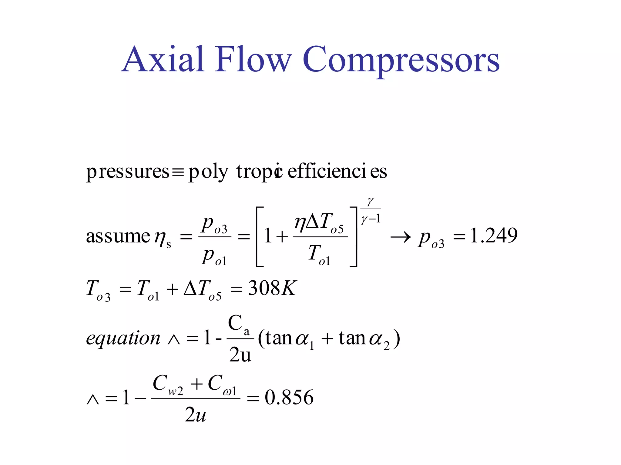
16. Axial Flow Compressors
)1/(
11
3
s
21
1213
12
12
11
2211
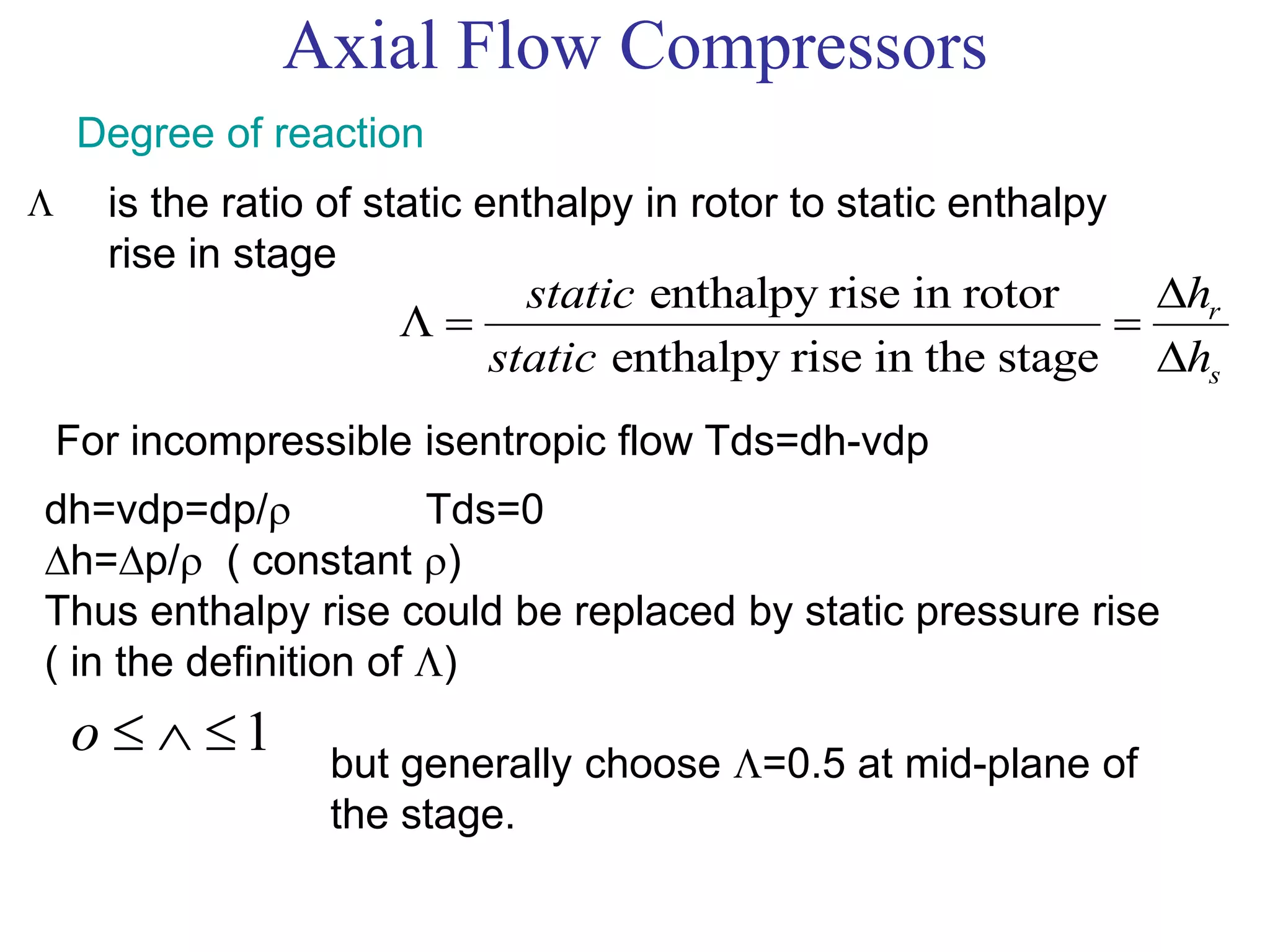
]1[R
stageperrisepressure
)tan(tan
)tan(tan
)tan(tan
)(
tantantantan













o
ss
o
o
p
a
ooooos
a
a
ww
a
T
T
p
p
c
UC
TTTTT
UCm
UCm
CCUmW
C
U




17. Axial Flow Compressors
 Design Process of an axial compressor
• (1) Choice of rotational speed at design point and annulus
dimensions
• (2) Determination of number of stages, using an assumed
efficiency at design point
• (3) Calculation of the air angles for each stage at the mean
line
• (4) Determination of the variation of the air angles from root
to tip
• (5) Selection of compressor blades using experimentally
obtained cascade data
• (6) Check on efficiency previously assumed using the
cascade data
• (7) Estimation on off-design performance
• (8) Rig testing

18. Axial Flow Compressors
 Design process:
• Requirements:
• A suitable design point under sea-level static conditions
(with =1.01 bar and , 12000 N as take off thrust, may
emerge as follows:
• Compressor pressure ratio 4.15
• Air-mass flow 20 kg/s
• Turbine inlet temperature 1100 K
• With these data specified, it is now necessary to
investigate the aerodynamic design of the compressor,
turbine and other components of the engine. It will be
assumed that the compressor has no inlet guide vanes,
to keep weight and noise down. The design of the
turbine will be considered in Chapter 7.

19. Axial Flow Compressors
 Requirements:
• choice of rotational speed and annulus dimensions;
• determination of number of stages, using an assumed
efficiency;
• calculation of the air angles for each stage at mean radius;
• determination of the variation of the air angles from root to
tip;
• investigation of compressibility effects

20. Axial Flow Compressors
 Determination of rotational speed and annulus
dimensions:
• Assumptions
• Guidelines:
• Tip speed Ut=350 m/s
• Axial velocity Ca=150-200 m/s
• Hub-tip ratio at entry 0.4-0.6
• Calculation of tip and hub radii at inlet
• Assumptions Ca=150 m/s
• Ut=350 m/s to be corrected to
250 rev/s
•

21. Axial Flow Compressors
 Equations
• continuity
thus
•
rpstt NtU ***2 
a
t
r
ta C
r
r
rACm















2
2
11 11

)(
1 2
2
11
2
a
r
r
C
m
r
t
r
a
t 












tr
t
rr
r
N /&rgettosolve,
2
350
t


2
.
2
1 1 r
t a
t
r
m r C
r
 
  
   
   

22. Axial Flow Compressors
procedure
31
1
1
1
11
2
1
1
1
1
/106.1
8.276
2
150C
bar01.1,288
11
2
1
1
1
mkg
RT
P
P
T
T
P
P
c
C
TT
C
PPKTT
oo
p
o
a
aoao



















23. Axial Flow Compressors
• From equation (a)
0.60.4/r
2/350
1
03837.0
r
2
2


















fromrassume
rtN
r
r
r
t
t
r
t

tr rr / N
260.60.21370.4
246.30.22620.5
227.50.24490.6
tr

24. Axial Flow Compressors
• Consider rps250
• Thus rr/rt=0.5, rt=0.2262, ut=2rt*rps=355.3 m/s
7.385V
2
1
2
11t  at CuGet
1RTa 
165.11
1 
a
v
M t
Is ok. Discussed later. Results r-t=0.2262,
r-r=0.1131, r-m=0.1697 m

25. Axial Flow Compressors
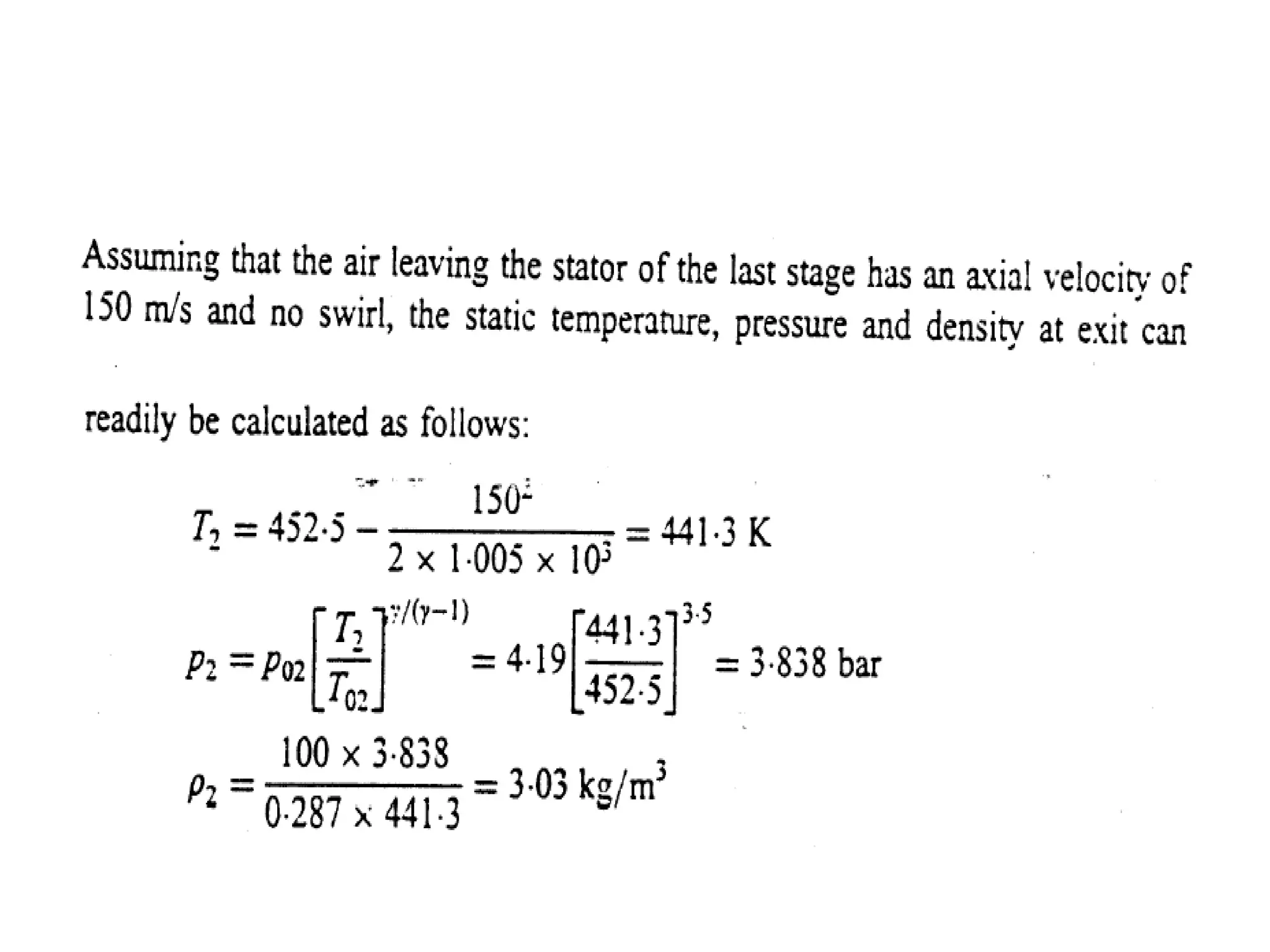
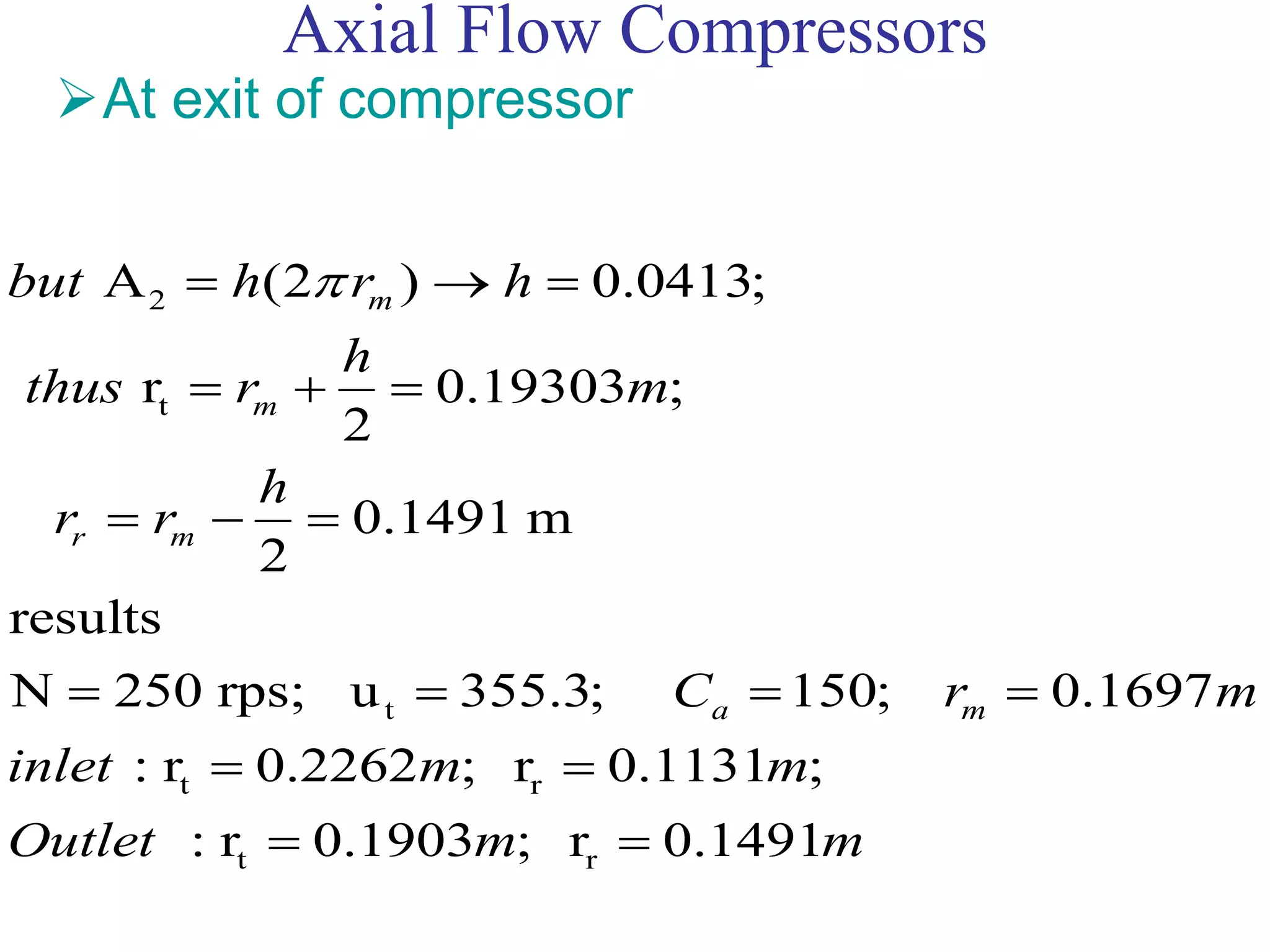
At exit of compressor
2 2 2
2
1 1 1
2
2 2
1
o
2
2 1
2 2
2
o
2
2 2
2
4.15 [ P 4.19 ];
n-1 1 0.4
where 317,
n 1.4
assume 0.9; 452.5 ;
P
441.3 K;
2 P
3.84 bar; 3.03 kg/
n
n
o o o
o o o
o
a
o
p o
P T P
given bar
P T P
T K
C T
T T
c T
P
P
RT









 
    
 
 
  
 
 
     
 
 
    3
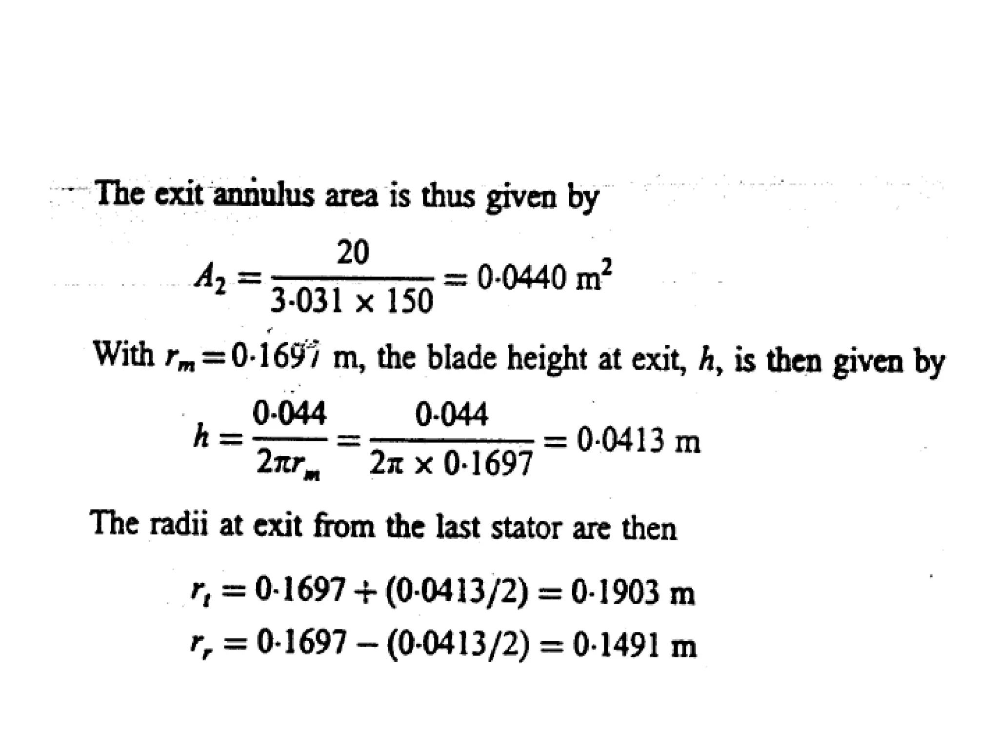
2 2 2
m ;
, A 0.044;am A C 

26. Axial Flow Compressors
At exit of compressor
2
t
t
t r
t r
A (2 ) 0.0413;
r 0.19303 ;
2
0.1491 m
2
results
N 250 rps; u 355.3; 150; 0.1697
: r 0.2262 ; r 0.1131 ;
: r 0.1903 ; r 0.1491
m
m
r m
a m
but h r h
h
thus r m
h
r r
C r m
inlet m m
Outlet m m
  
  
  
   
 
 

27. Axial Flow Compressors
No. of stages
• To =overall = 452.5-288=164.5K
• rise over a stage 10-30 K for subsonic
• 4.5 for transonic
• for rise over as stage=25
• thus no. of stages =164.5/25 stages7
- normally To5 is small at first stage
de haller criterion V2/V1 > 0.72
-work factor can be taken as 0.98, 0.93, 0.88 for 1st,
2nd, 3 rd stage and 0.83 for rest of the stages.

28. Axial Flow Compressors
 Stage by stage
design;
• Consider middle plane
• stage 1
• for no vane at inlet
wo CuT  cp
0,/9.76 1  smCw
smCC ww /9.76,0 21 
m/s266uthus,r2u mm  

29. Axial Flow Compressors
• Angles
o
a
w
a
w
a
thus
C
C
C
Cu
C
u
98.8
bladesrotorindeflectionthe
14.27tan
67.51tan
64.60tan
21
2
2
2
2
2
2
11










check de Haller
0.72thanlessiswhich79.0
cos
cos
cos
cos/
2
1
1/
2
1
2





a
a
C
C
v
v

30. Axial Flow Compressors
856.0
2
1
)tan(tan
2u
C
-1
308
249.11assume
esefficiencicpoly tropipressures
12
21
a
513
3
1
1
5
1
3
s










 



u
CC
equation
KTTT
p
T
T
p
p
w
ooo
o
o
o
o
o







31. Axial Flow Compressors
• Second stage
05.41;06.11
tantan;tantan
7.42&7.57(b)and(a)
)(488.2tantan
7.0take);tan(tan
2
)2(
)(6756.0tantan
)tan(tanc)1(
93.0,25
21
22
2
1
0
21
21
21
21
215p
5
















aa
a
ao
o
C
u
C
u
solve
b
u
C
a
uCT
KT

32. Axial Flow Compressors
0.28;24.51
)tan(tan
2
);tan(tan
5.0,25T0.88,
3
907.0
06.11cos
15.27cos
cos
cos
721.0
cos
cos
V
V
;stagesecondfor
bar599.1
308
25
1
33325308
21
21215
03
1
2
2
3
2
1
1
2
3
5.3
3
1
3





















solving
u
C
uCTc
K
stage
C
C
Hallerde
p
P
P
T
a
aop
o
s
o
o
o

33. Axial Flow Compressors
  Kp
eperformanc
givingthus
take
o 35724333Tbar;992.1246.1599.1)(
246.1
333
249.0
1
p
p
stagerd3of*
0.718ofnumberHallerde;65.28,92.50
685.0tantan24T
709.0
28cos
24.51cos
cos
cos
isno.Hallerde
3o33
5.3
3o1
o
21
21o5
2
1
3






 
















34. Axial Flow Compressors
:belowsummerizedbecanstagesthreetheofeperformanc
).(71.2738.51
7773.1
150
6.266
25.0)tan(tan
7267.0
1506.26683.0
10005.124
tantan;1
)tan(tan
2
)tan(tanc
5,6and4stages
/7.18492.50tan150;/9.8163.28tan150C
bygivenaresvelocitiewhirlthe.92.50
63.28diagramvelocitytheofsymmetryFrom
12
0
1
21
3
21
21215p
21
0
12
21
1
5
1
3
the
andyielding
T
T
p
p
u
C
uCT
smCsm
and
o
o
o
o
a
ao



















 






35. Axial Flow Compressors
1oT
1
3
o
o
p
p
13 oo pp 
3oT
3op
1oP
654Stage
2.9682.4471.992
405381357
1.1991.2131.228
3.5602.9682.447
429405381
0.5920.5210.455

36. Axial Flow Compressors
• Stage 7
• At entry to the final stage the pressure and
temperature are 3.56 bar and 429 K. the required
compressor delivery pressure is 4.15*1.01=4.192 bar.
The pressure ratio of the seventh stage is thus given
by
KTgiving
th
p
p
os
o
o
8.22
177.1
429
T0.90
1
fromdetrminedbecanratiopressurethe
givetorequiredriseretemperatue
177.1
56.3
192.4
5.3
os
71
3






 








37. Axial Flow Compressors
• the corresponding air angles, assuming 50 per cent
reaction, are then 1=50.98,
0.717.ofnumberHallerde
rysatisfactoa)(52.28 1
0
2 with 

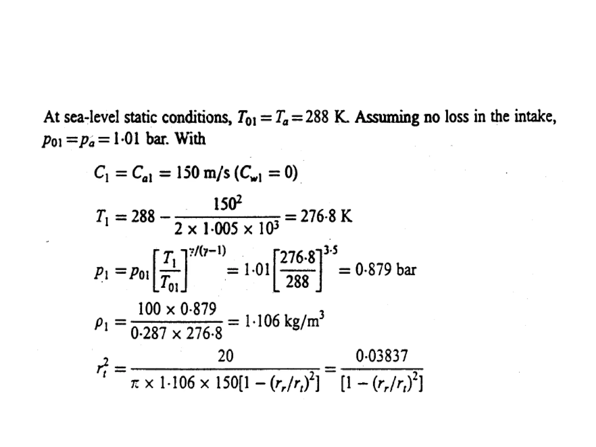
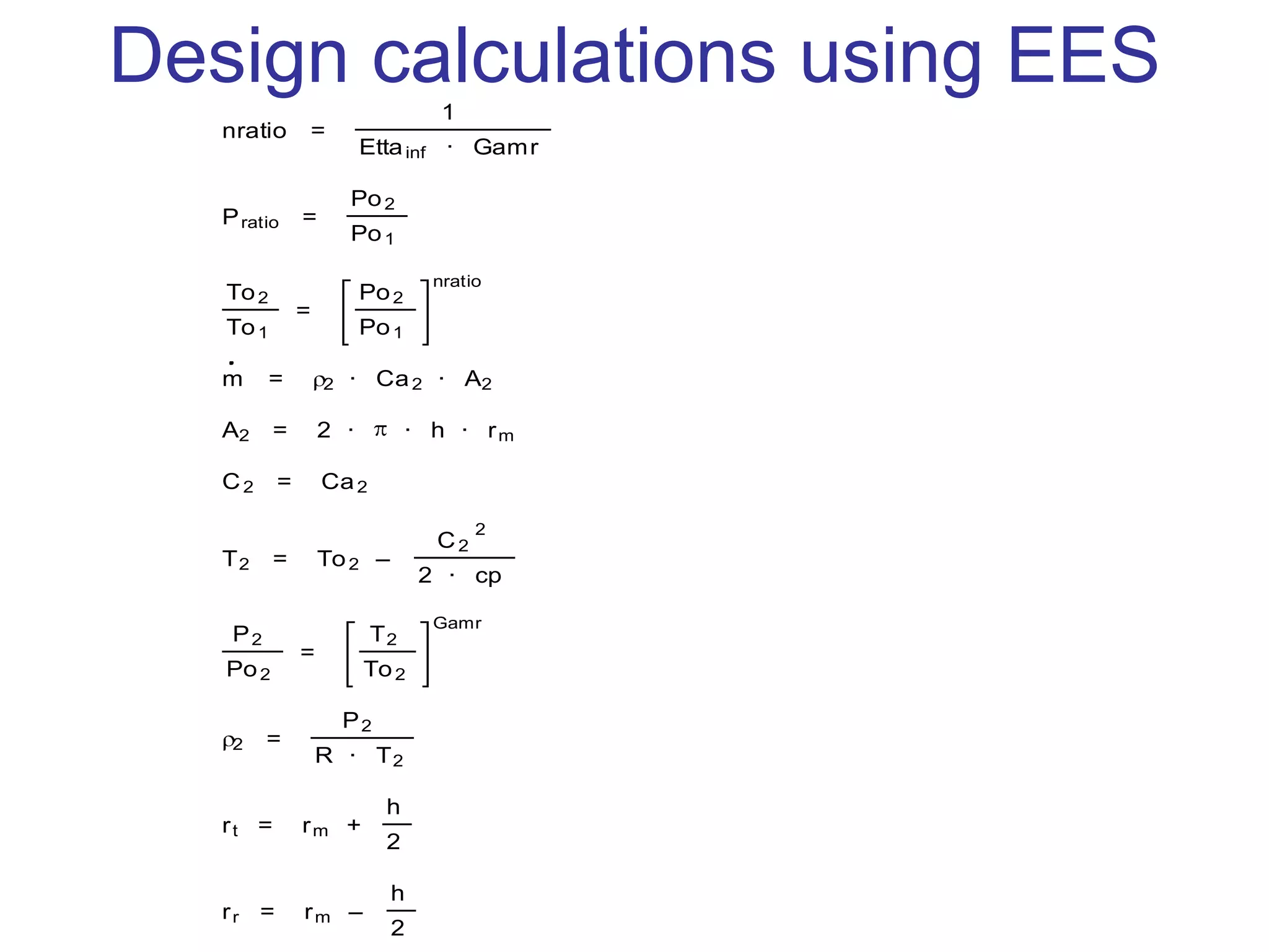
38. Design calculations using EES
– "Determination of the rotational speed and annulus dimensions"
– "Known Information"
– To_1=288 [K]; Po_1=101 [kPa]; m_dot=20[kg/s]; U_t=350 [m/s]
– $ifnot ParametricTable
– Ca_1=150[m/s];r_r/r_t=0.5;cp=1005;R=0.287;Gamma=1.4
– $endif
– Gamr=Gamma/(Gamma-1)
– m_dot=Rho_1*Ca_1*A_1 "mass balance"
– A_1=pi*(r_t^2-r_r^2)"relation between Area and eye dimensions"
– U_t=2*pi*r_t*N_rps
– C_1=Ca_1
– T_1=To_1-C_1^2/(2*cp)
– P_1/Po_1=(T_1/To_1)^Gamr
– Rho_1=P_1/(R*T_1)
– $TabStops 0.5 2 in

39. Design calculations using EES
Determination of the rotational speed and annulus dimensions
Known Information
To1 = 288 [K] Po1 = 101 [kPa] m = 20 [kg/s] Ut = 350 [m/s]
Ca1 = 150 [m/s] rr
rt
= 0.5
cp = 1005 R = 0.287 = 1.4
Gamr =
– 1
m = 1 · Ca1 · A1 mass balance
A1 = · ( rt
2
– rr
2
) relation between Area and eye dimensions
Ut = 2 · · rt · Nrps
C1 = Ca1
T1 = To1 –
C1
2
2 · cp
P1
Po1
=
T1
To1
Gamr
1 =
P1
R · T1

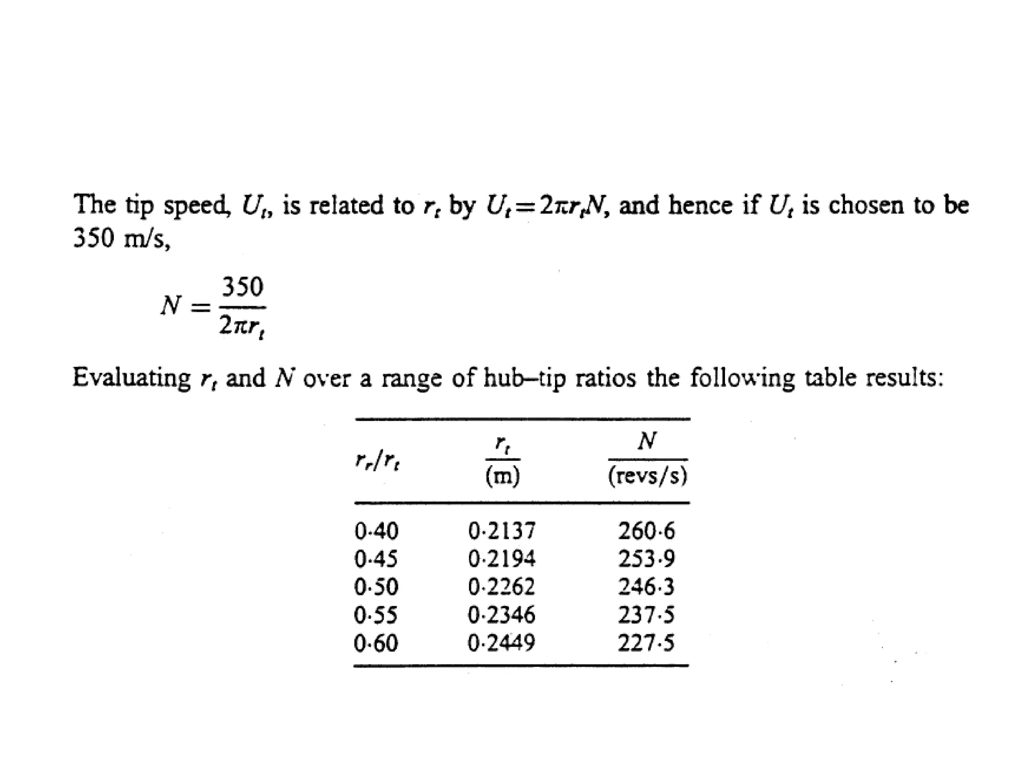
40. Design calculations using EES
Calculate radii at exit section
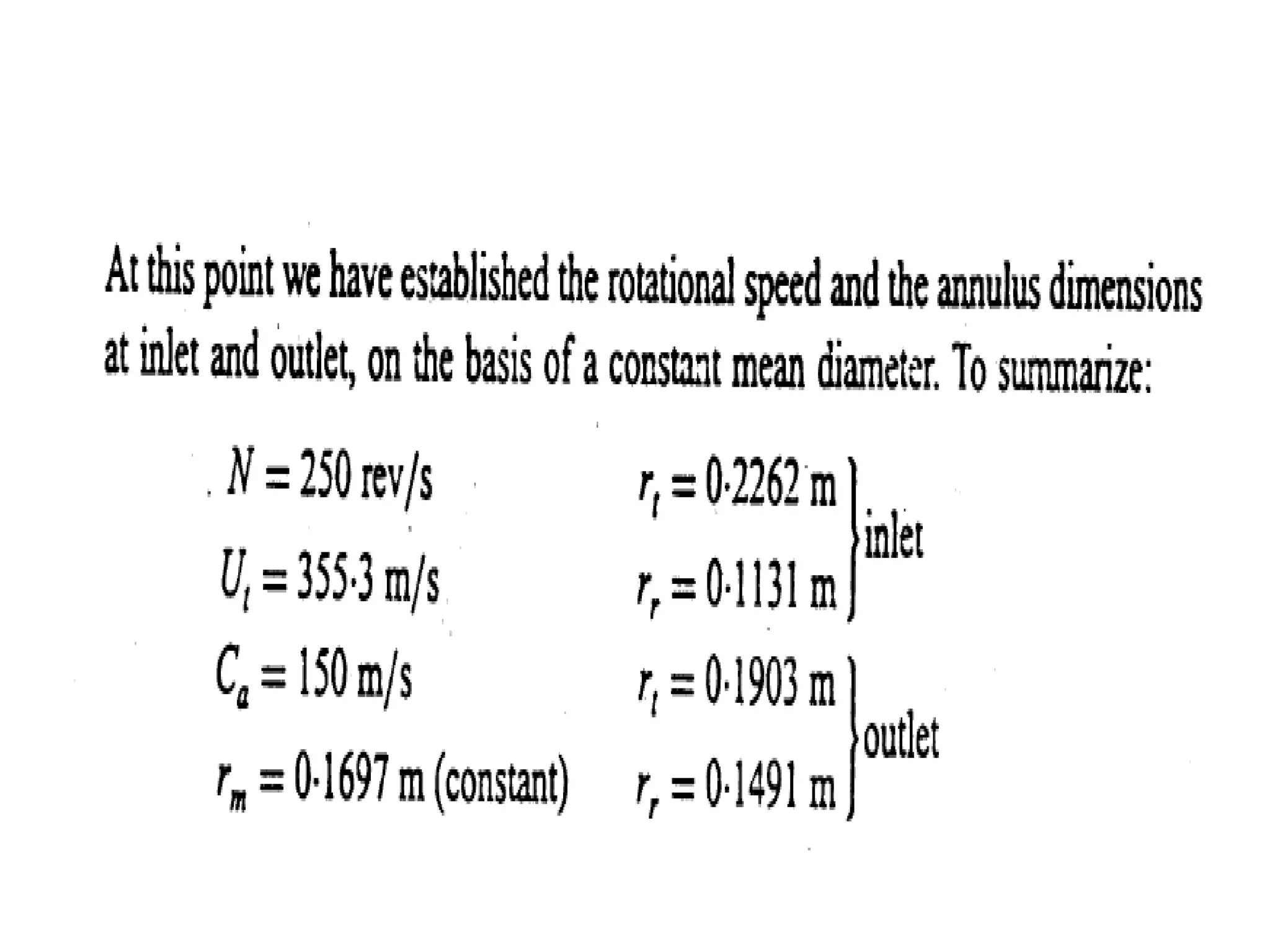
Choose (round) rotational speed as 250 rps
Nrps = 250
Thus calc new value for tip speed
rt1 = 0.2262
Ut = 2 · · rt1 · Nrps
rm = 0.1697
Known Information
To1 = 288 [K]
Pratio = 4.15
Assumptions
Ettainf = 0.9
Ca2 = Ca1
Ca1 = 150 [m/s]
Gamr =
– 1

41. Design calculations using EES
nratio =
1
Ettainf · Gamr
nratio=(n-1)/n=(1/ettainf )/ga
Pratio =
Po2
Po1
To2
To1
=
Po2
Po1
nratio
m = 2 · Ca2 · A2
A2 = 2 · · h · rm
C2 = Ca2
T2 = To2 –
C2
2
2 · cp
P2
Po2
=
T2
To2
Gamr
2 =
P2
R · T2
rt = rm +
h
2
rr = rm –
h
2

42. Design calculations using EES
A2 = 0.04398 Ca1 = 150 [m/s] Ca2 = 150 [m/s] cp = 1005 [J/kgK] C2 = 150 [m/s] Ettainf = 0.9
= 1.4 Gamr = 3.5 h = 0.041 [m] m = 20 [kg/s] nratio = 0.3175 Nrps = 250 [revper sec]
Po1 = 101 [kPa] Po2 = 419.2 P2 = 384 [kPa] Pratio = 4.15 R = 0.287 [kJ/kgK] 2 = 3.032
rt1 = 0.2262 [m] rm = 0.1697 [m] rr = 0.1491 [m] rt = 0.1903 [m] To1 = 288 [K] To2 = 452.5 [K]
T2 = 441.3 [C] Ut = 355.3 [m/s]

43. Design calculations using EES
Calculate number of stages
Known Information
To1 = 288 [K] Po1 = 101 [kPa] m = 20 [kg/s]
Pratio = 4.15 Tooutlet = 452.5
Assumptions
delTstage = 25
Ca1 = 150 [m/s] cp = 1005 R = 0.287 = 1.4
Gamr =
– 1
delTov = Tooutlet – To1
Nstages =
delTov
delTstage

44. Design calculations using EES
Ca1 = 150 [m/s] cp = 1005 [J/kgK] delTov = 164.5 delTstage = 25 = 1.4 Gamr = 3.5 m = 20 [kg/s] Nstages = 6.58
Po1 = 101 [kPa] Pratio = 4.15 R = 0.287 [kJ/kgK] To1 = 288 [K] Tooutlet = 452.5