Downloaded 109 times

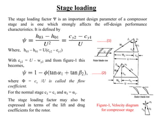
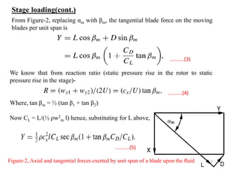


The document explores the design and performance characteristics of axial flow compressors and fans, focusing on the stage loading factor, flow coefficients, and off-design performance influences. It discusses the efficiency, pressure rise, and loss factors in compressor stages and provides equations for various calculations related to compressor performance. Additionally, it includes concepts of stability in compressors and the application of blade element theory in fan design.


