Download as PDF, PPTX


![Proportionality factors
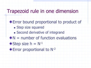
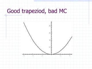
Error bound in classical methods
depends on maximum of derivatives.
MC error proportional to variance of
function, E[f2] – E[f]2](https://image.slidesharecdn.com/mcqmc-100510110351-phpapp02/85/Monte-Carlo-and-quasi-Monte-Carlo-integration-10-320.jpg)


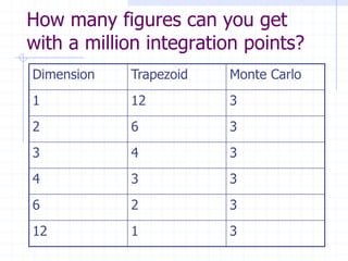
This document discusses Monte Carlo and quasi-Monte Carlo integration methods. It explains that while classical integration rules like the trapezoid rule become less accurate in higher dimensions, Monte Carlo integration maintains the same error rate regardless of dimension. Quasi-Monte Carlo sequences can converge even faster than Monte Carlo, though the rate depends on the specific sequence used. The document provides examples of integration methods and sequences, and discusses factors that affect the performance and accuracy of Monte Carlo, quasi-Monte Carlo, and lattice rule integration techniques.