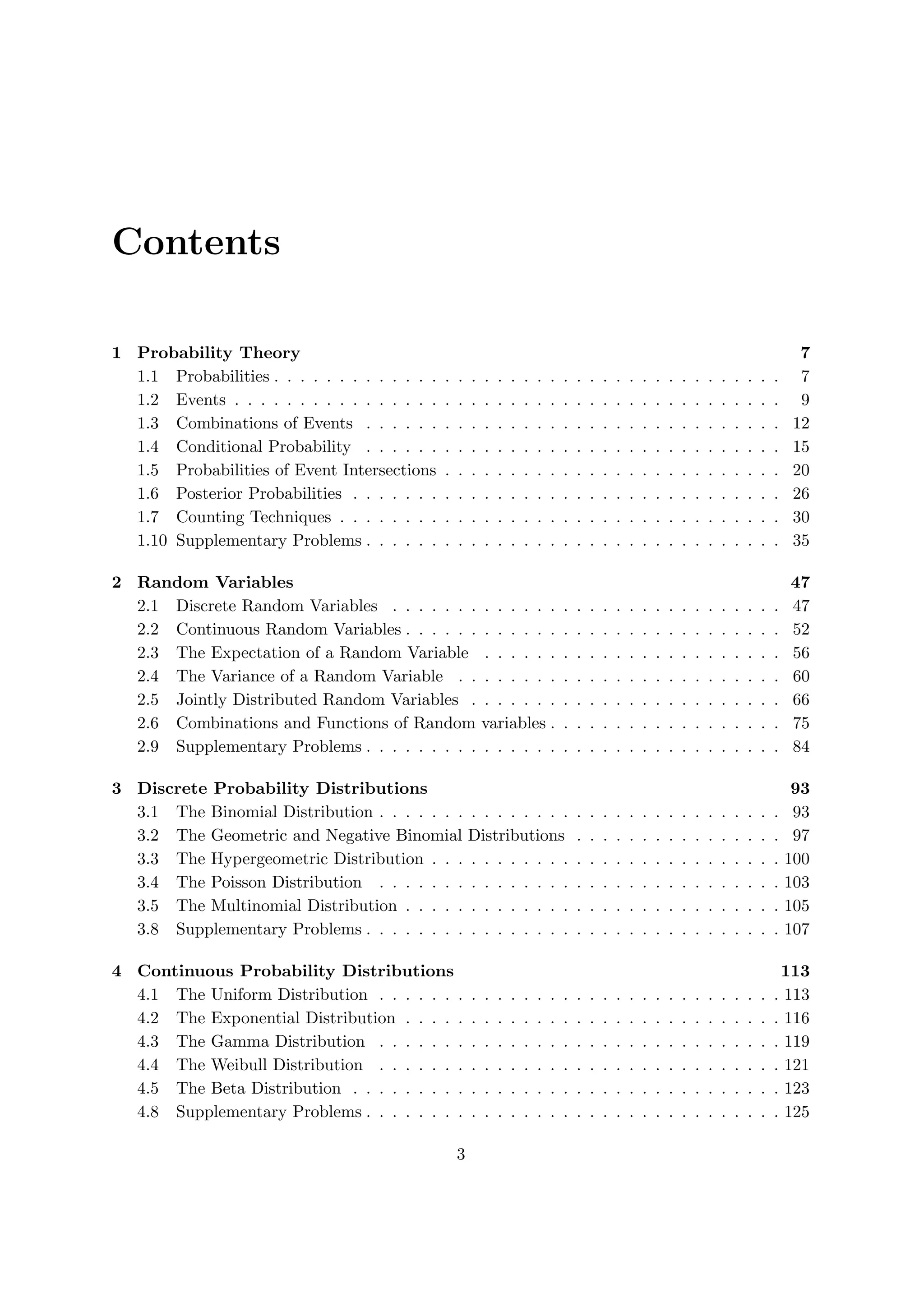
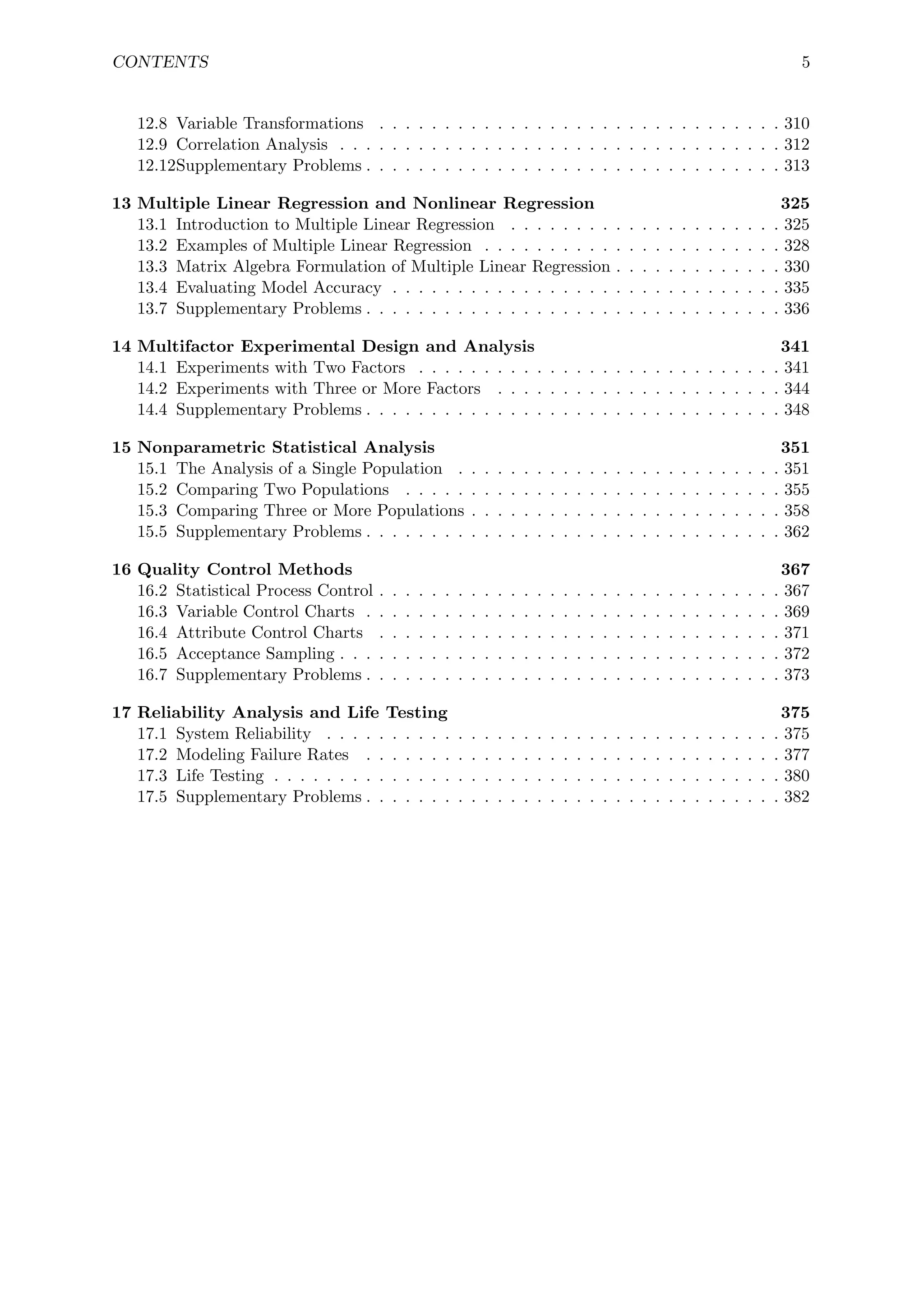
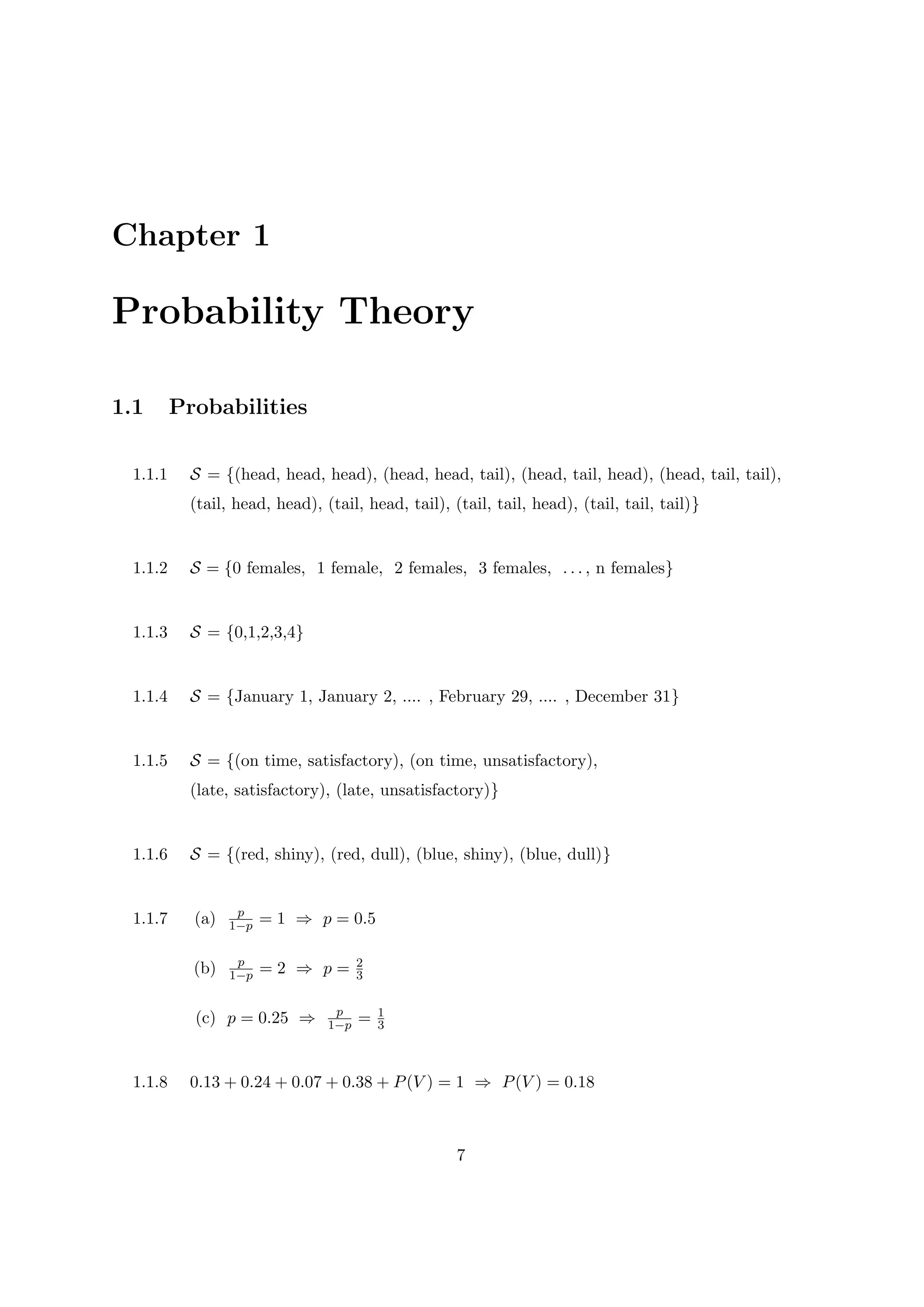
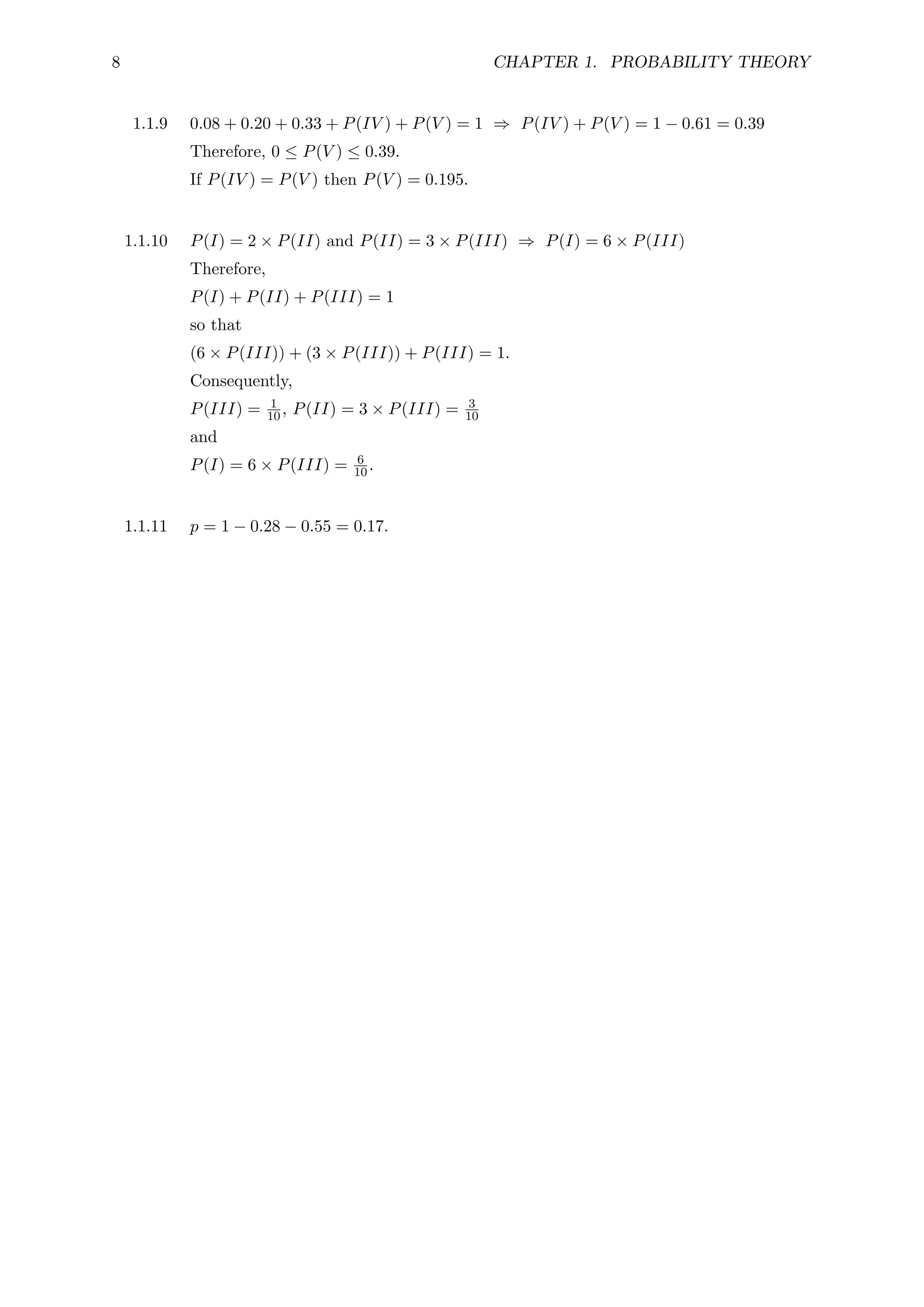
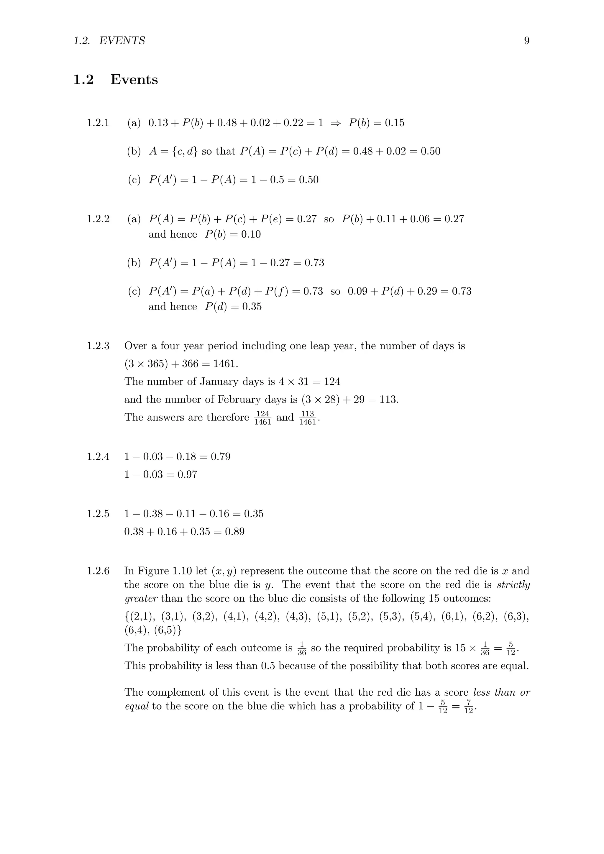
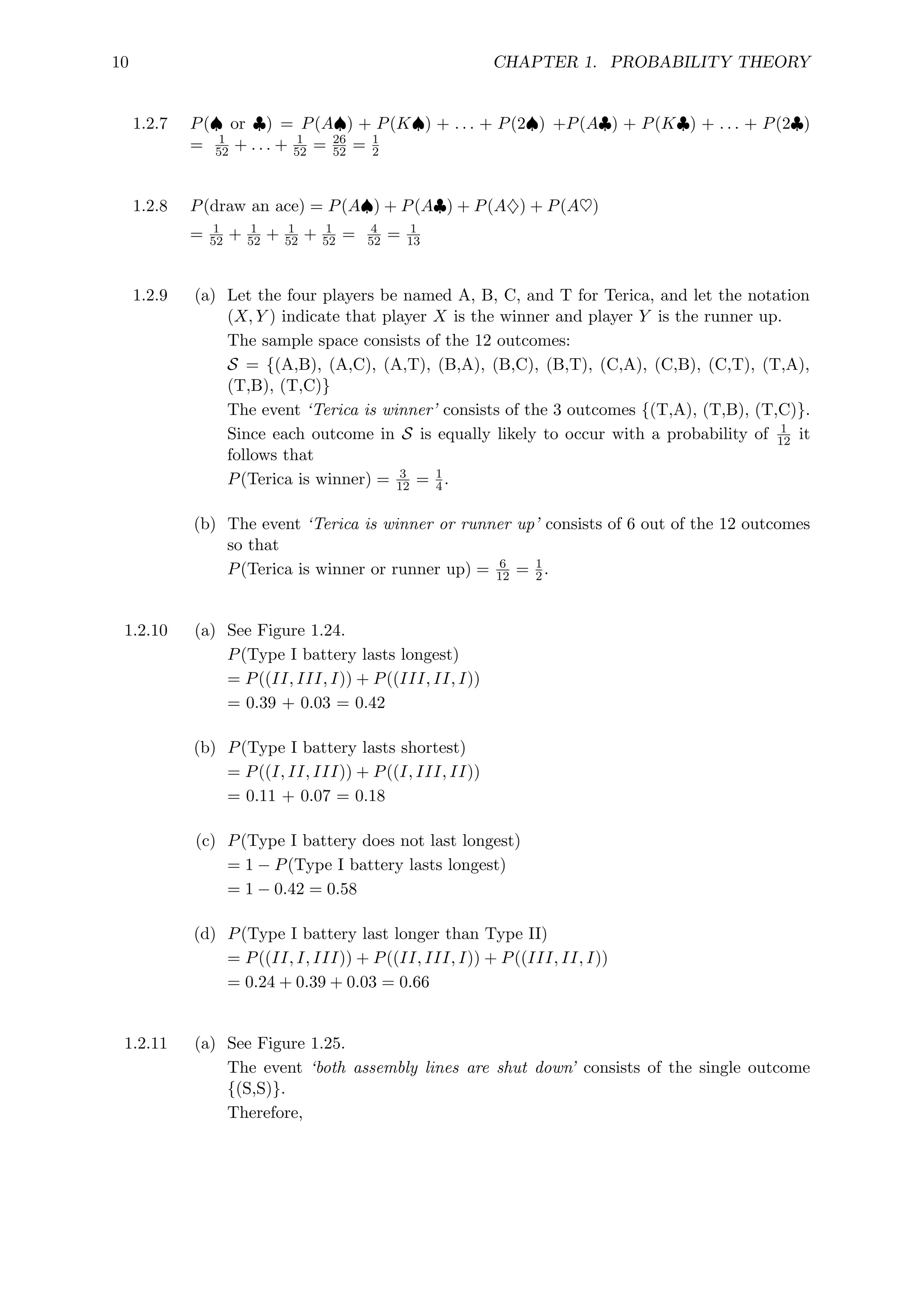
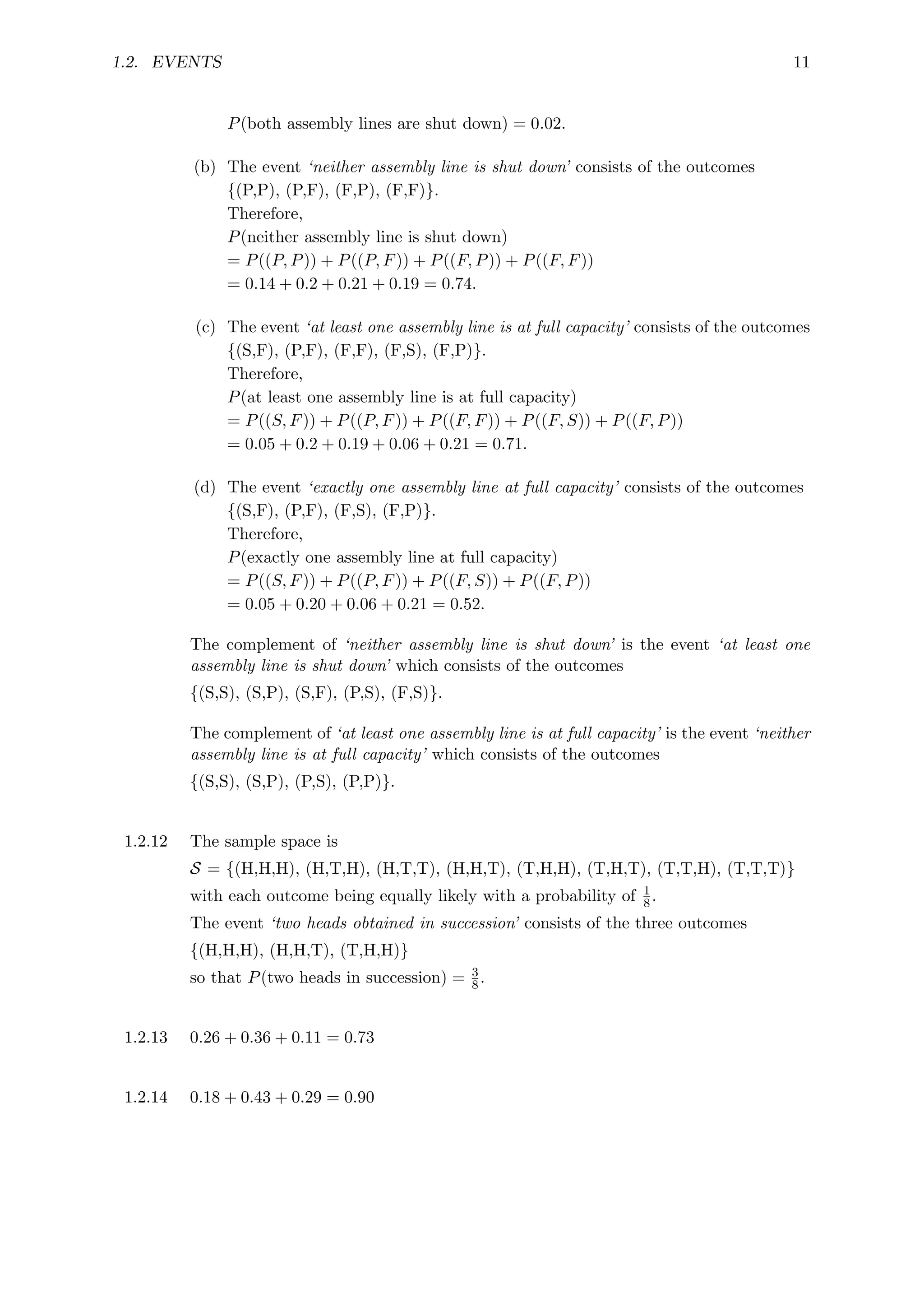
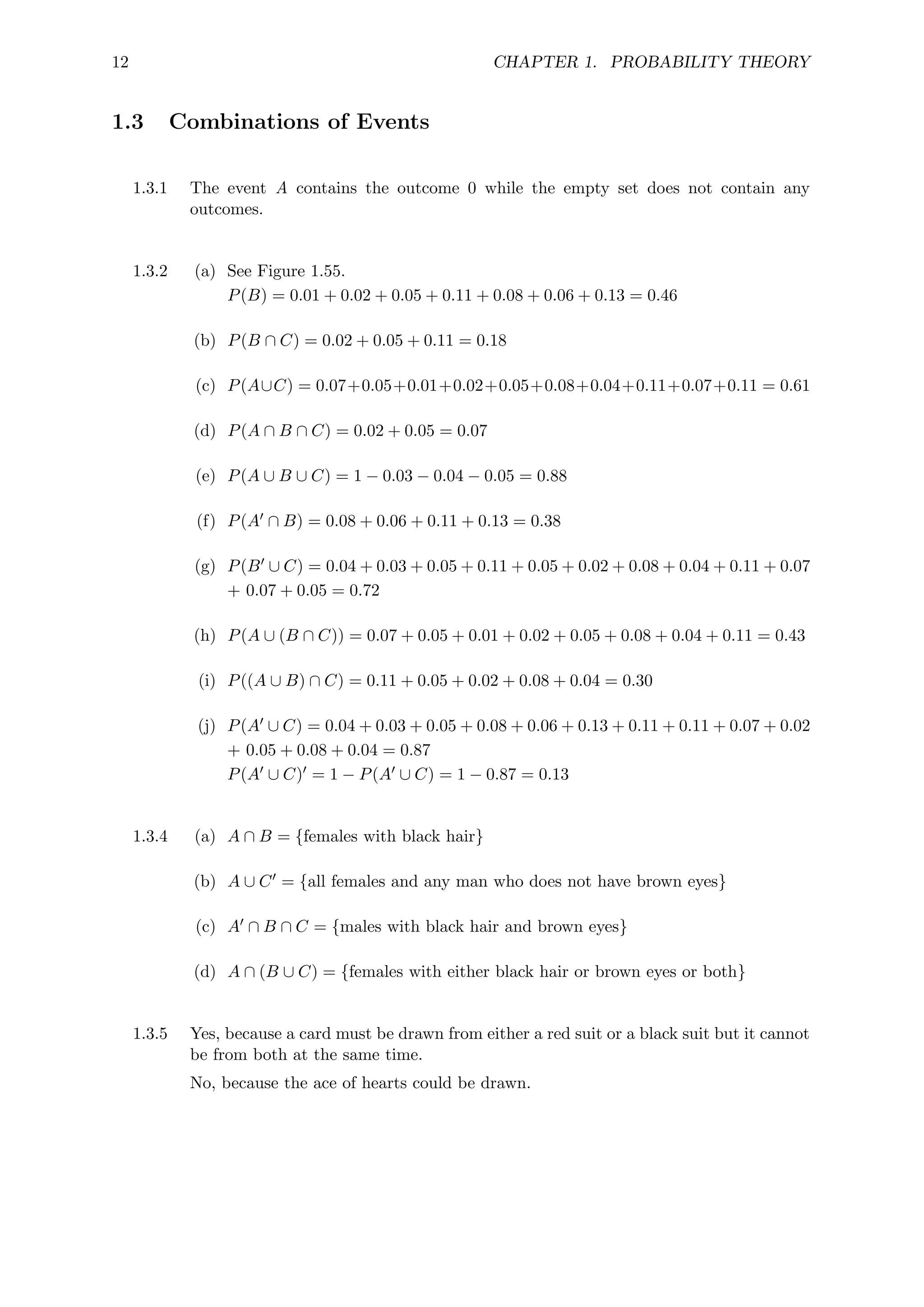
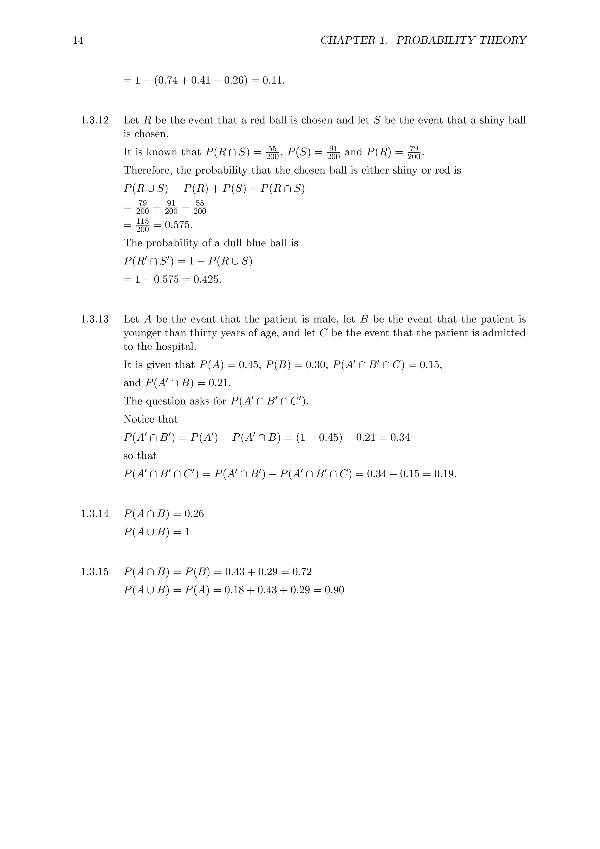
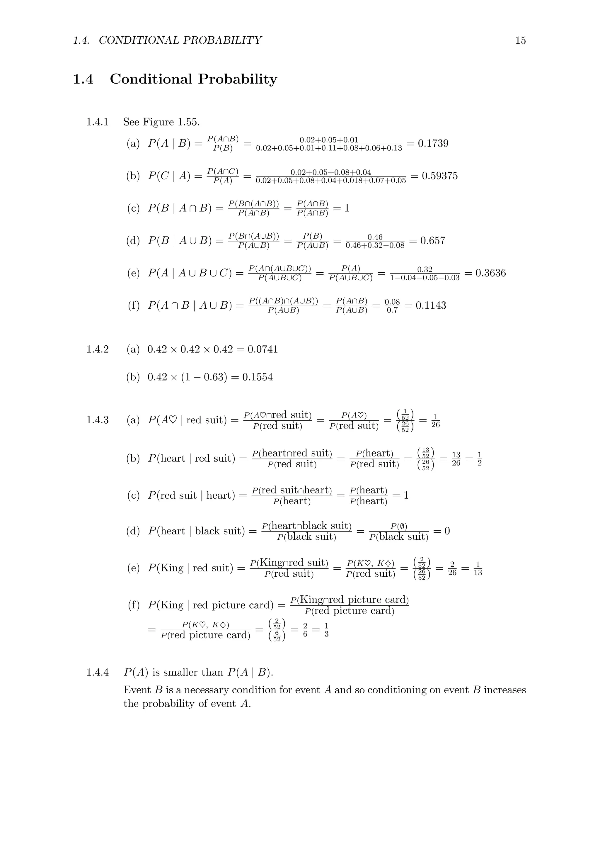
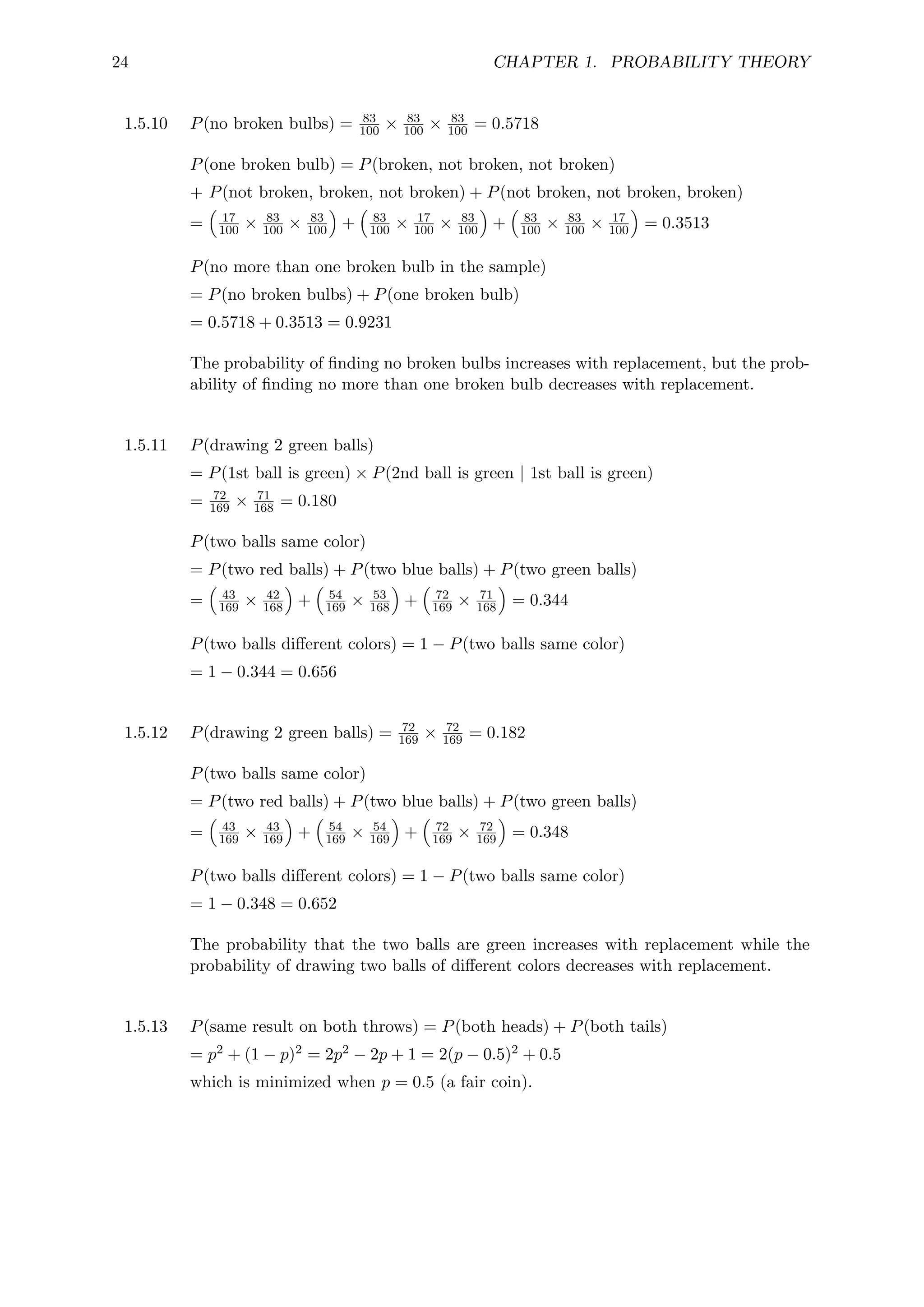
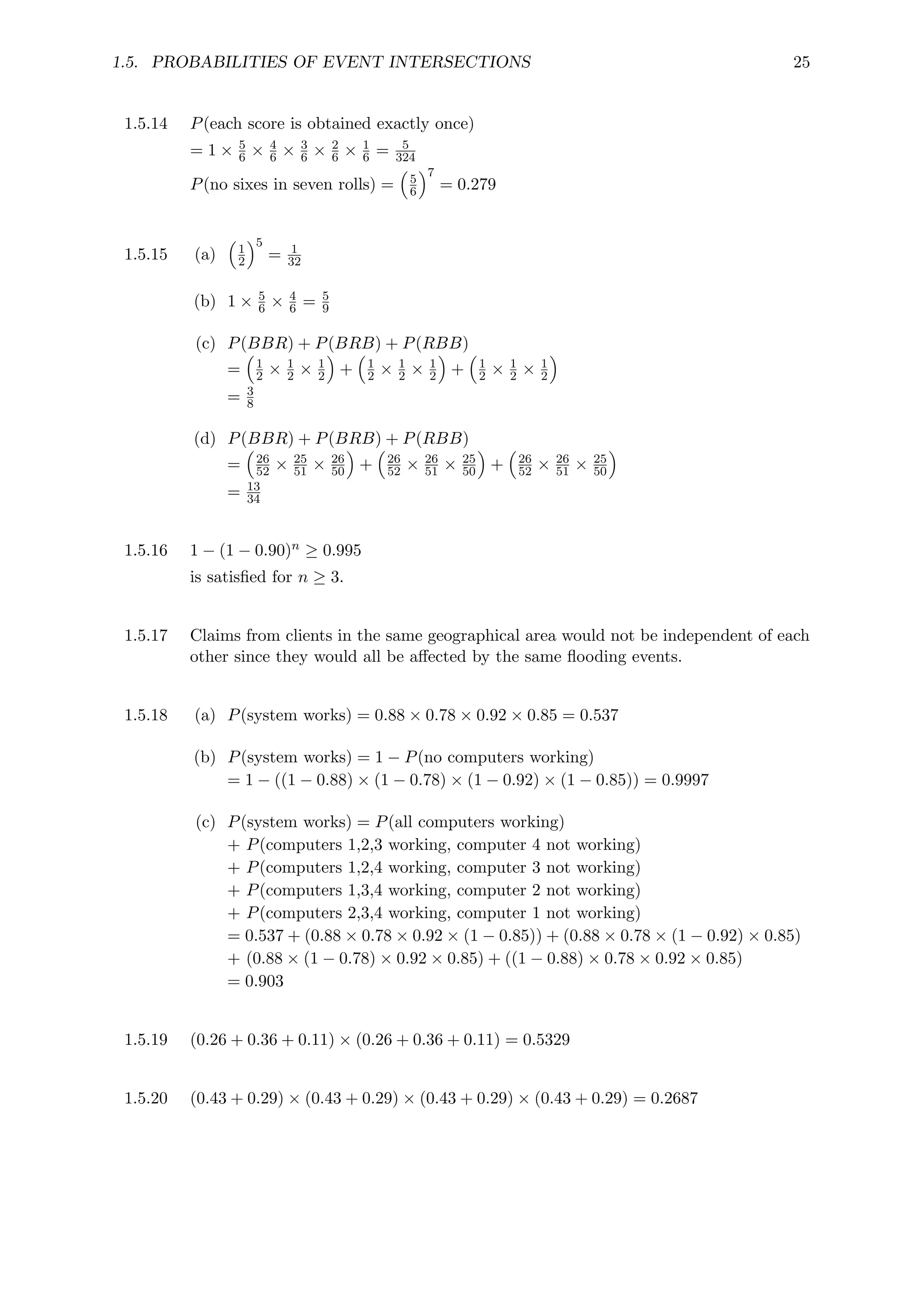
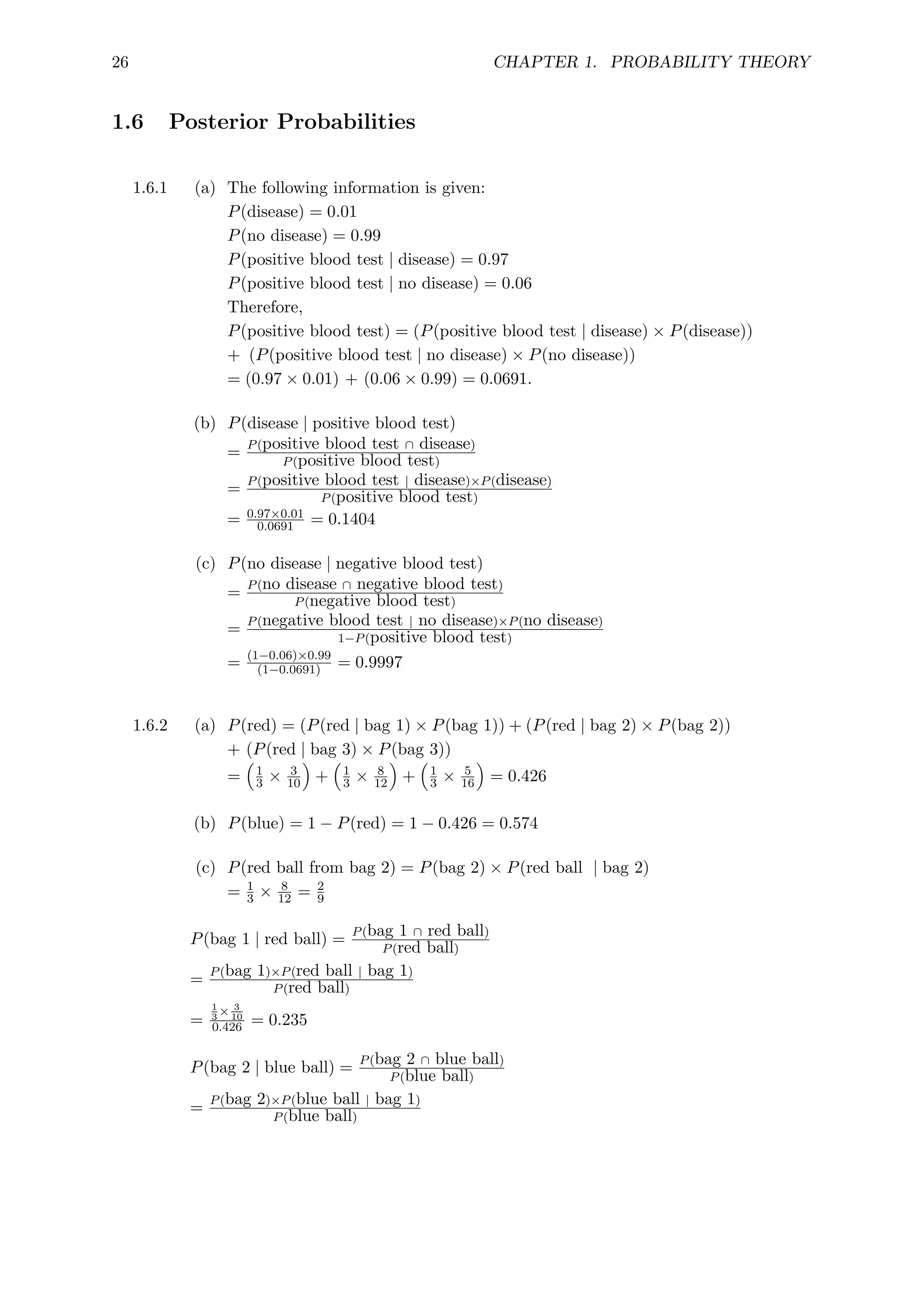
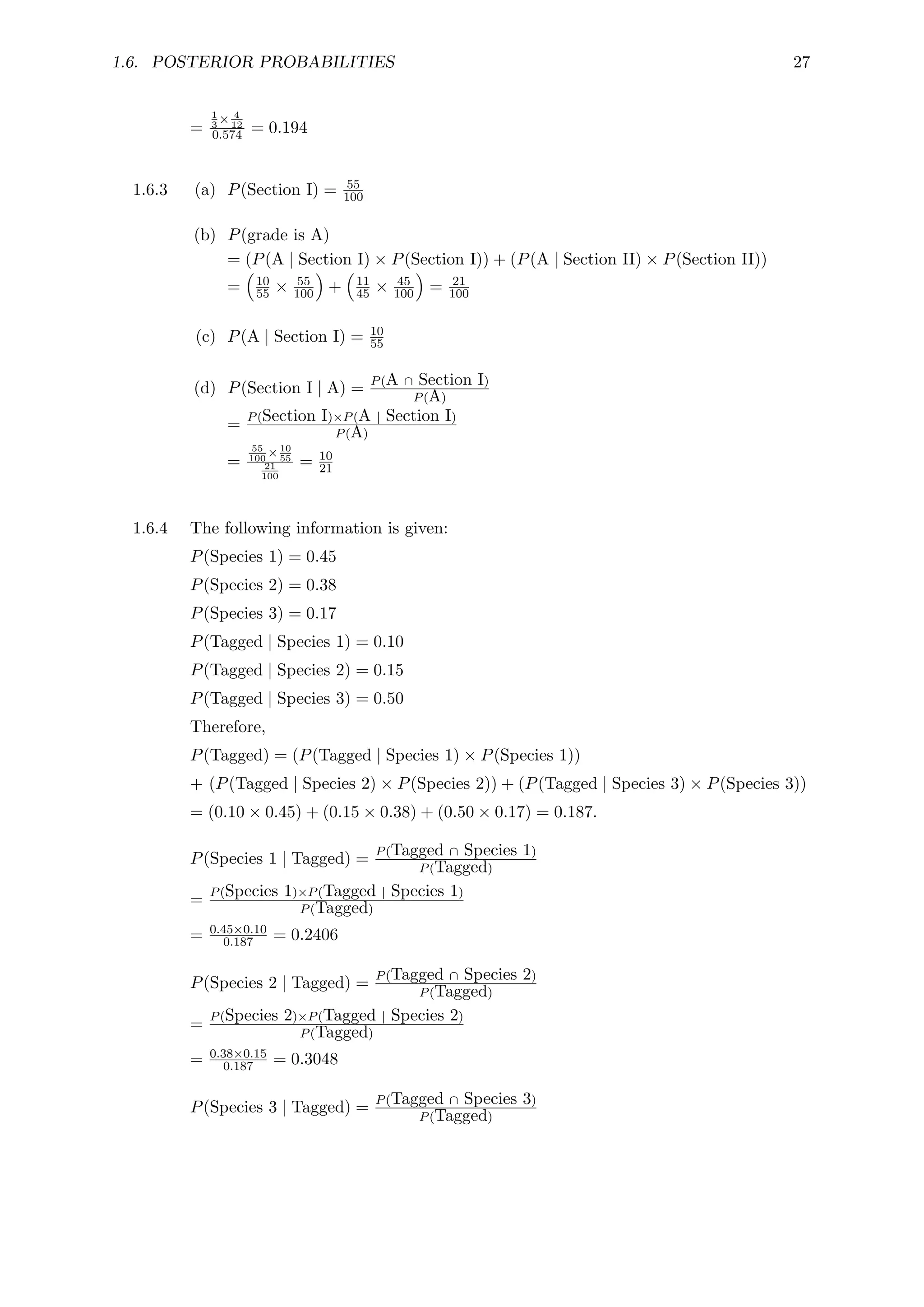
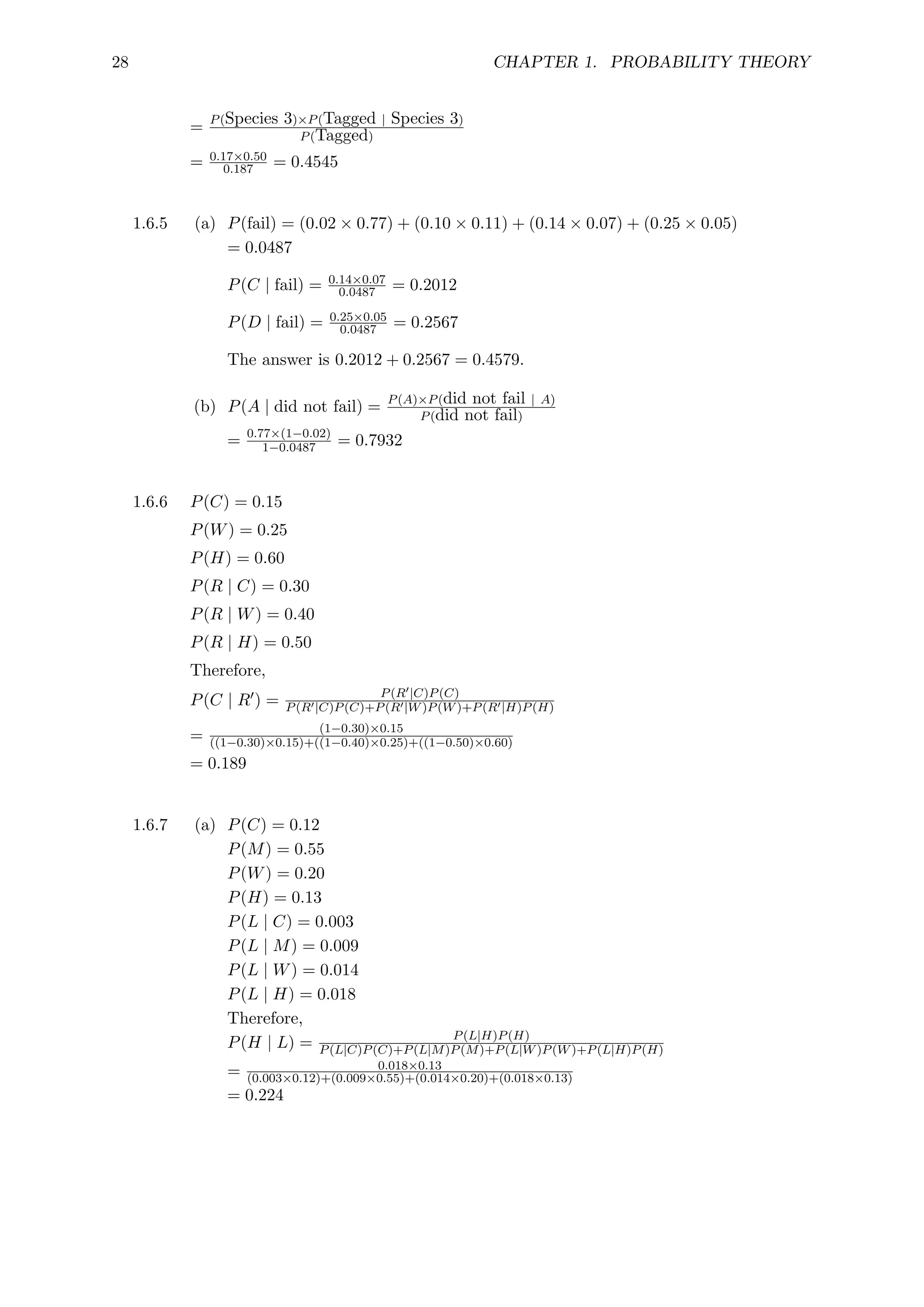
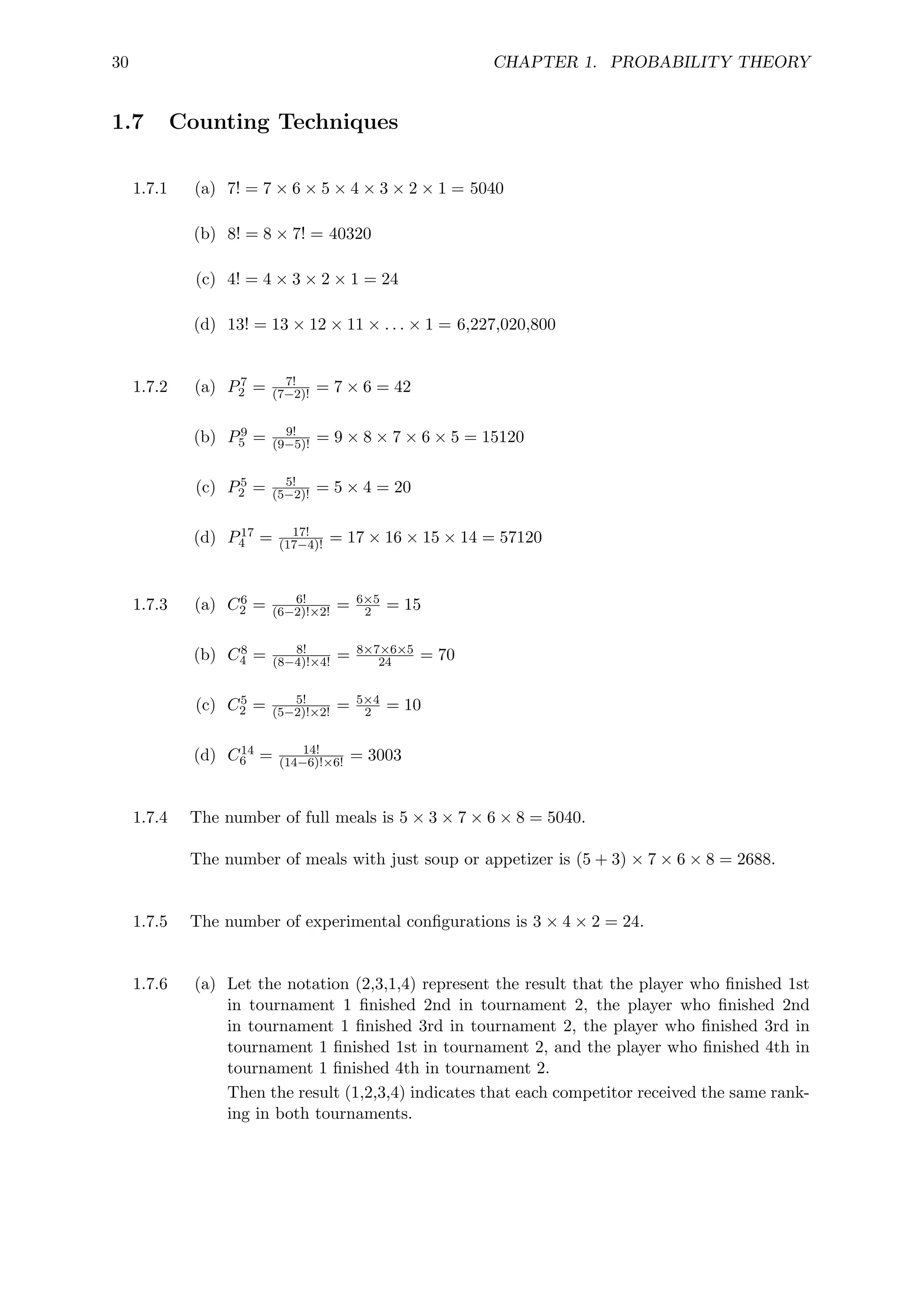
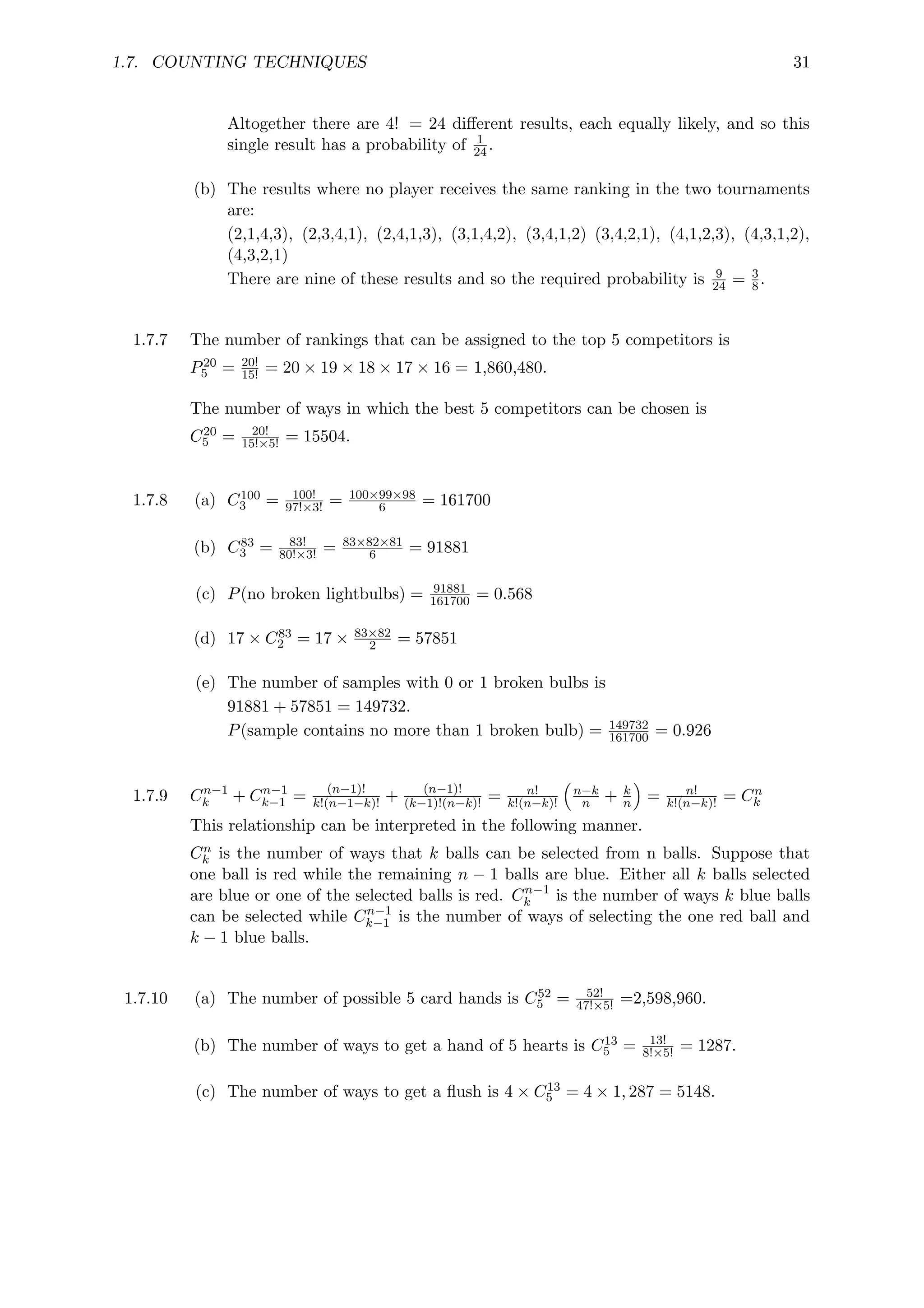
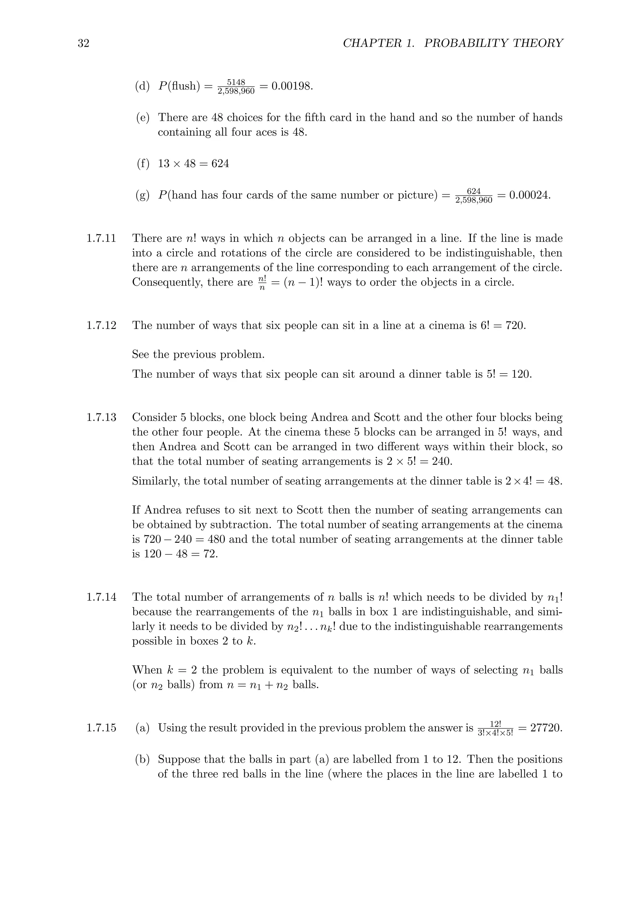
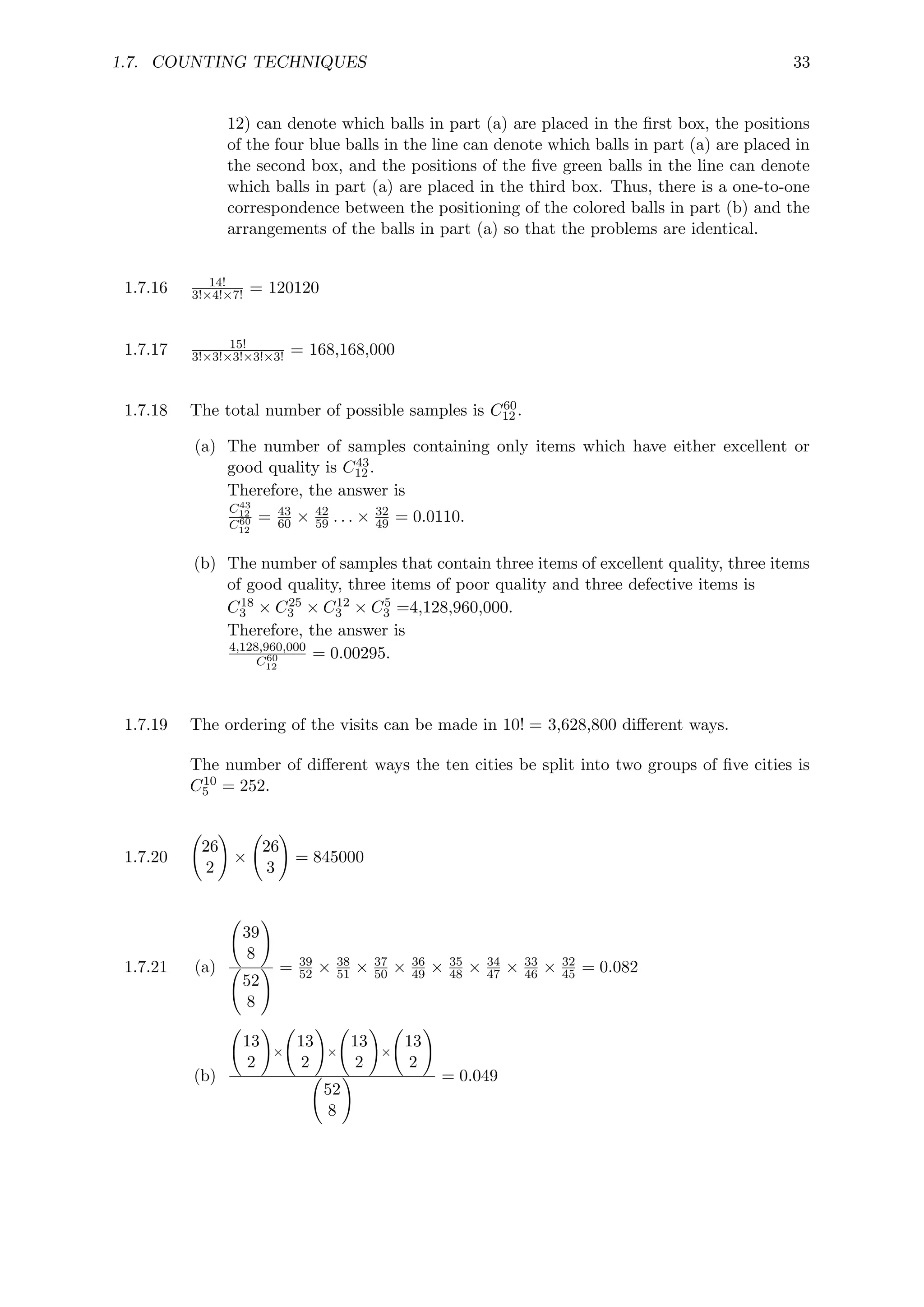
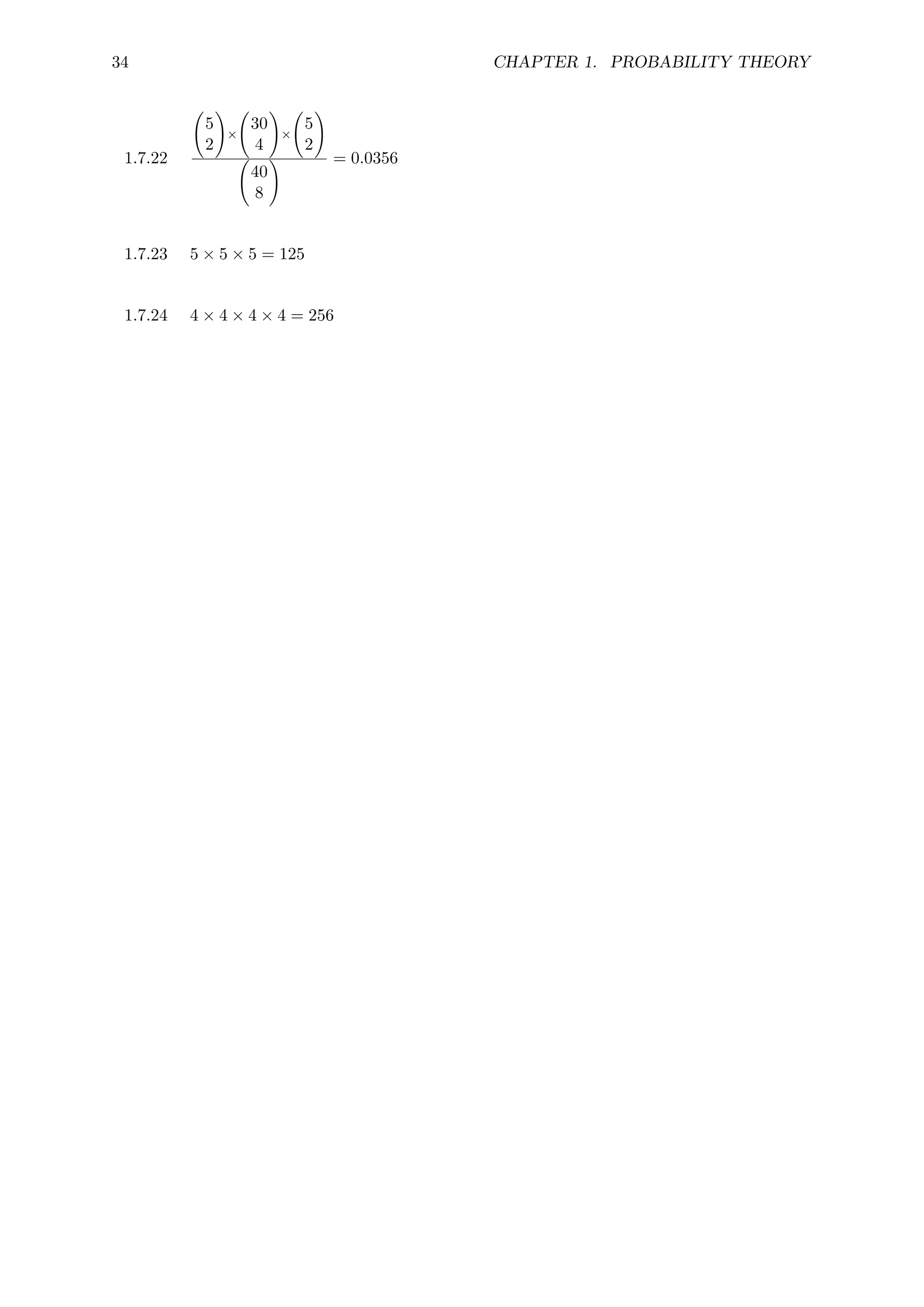
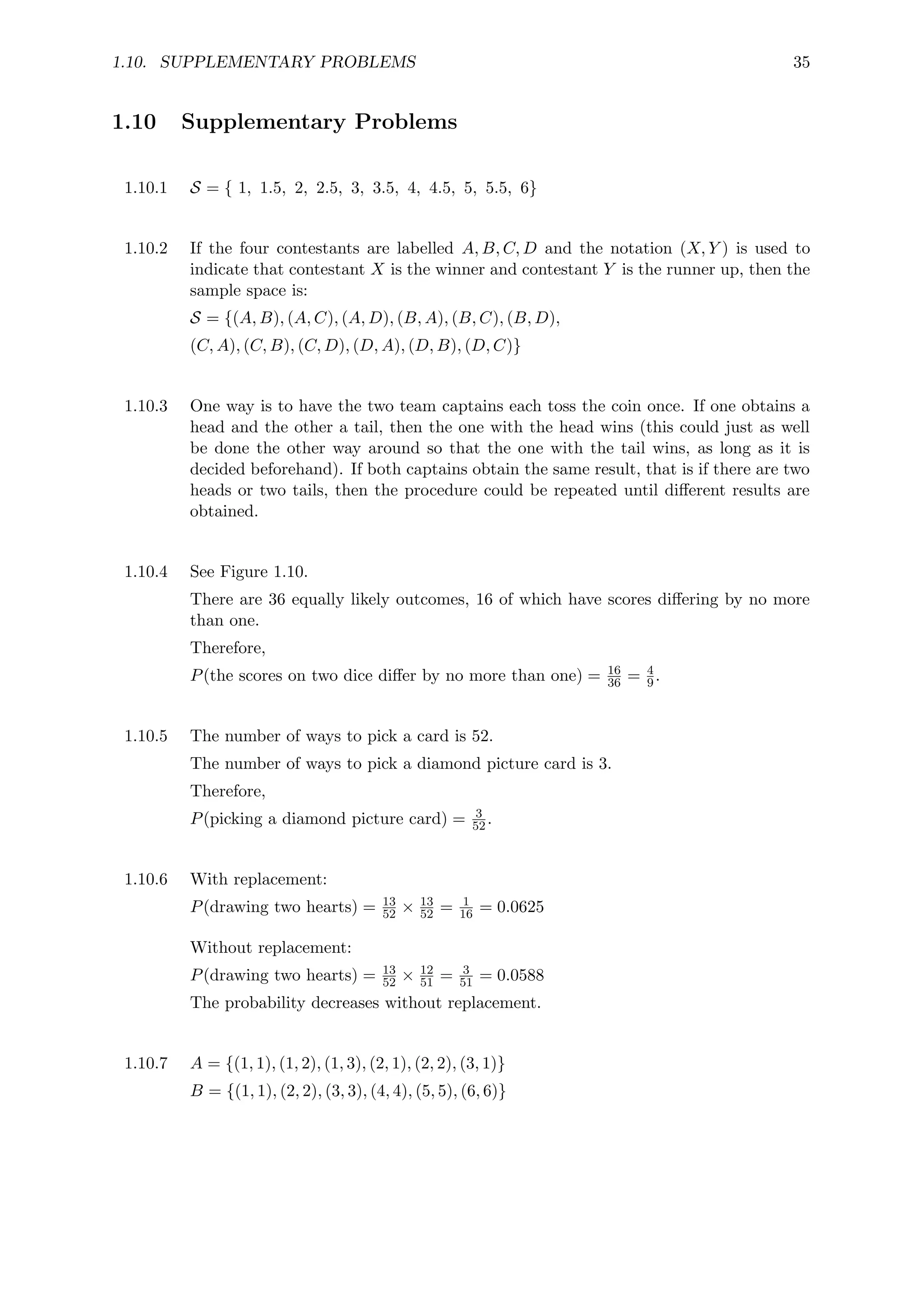
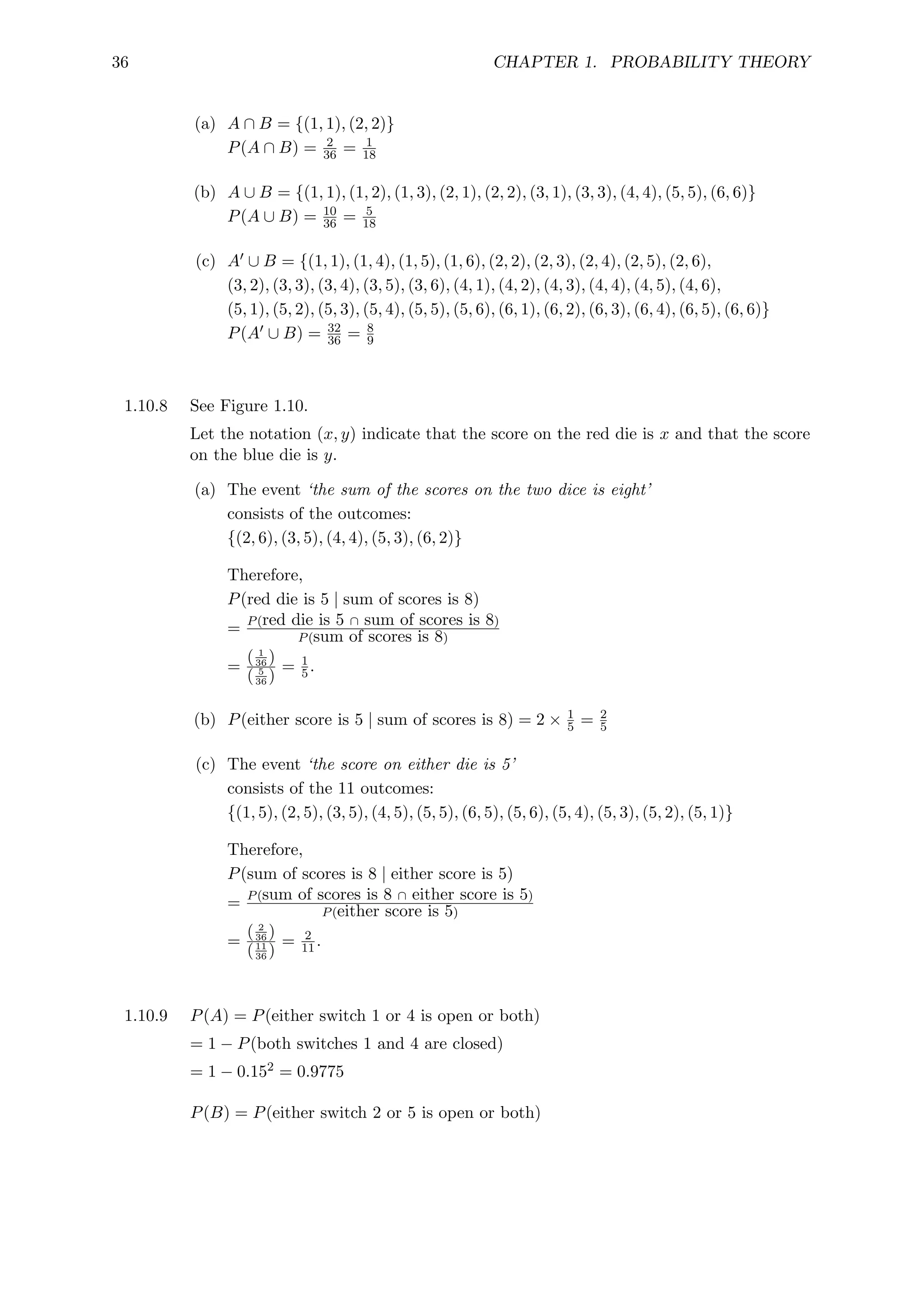
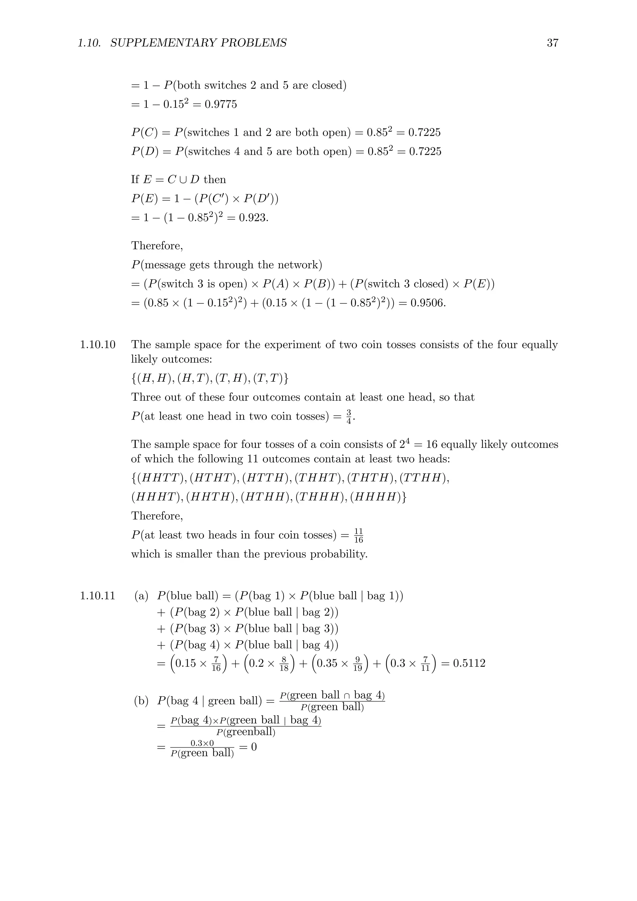
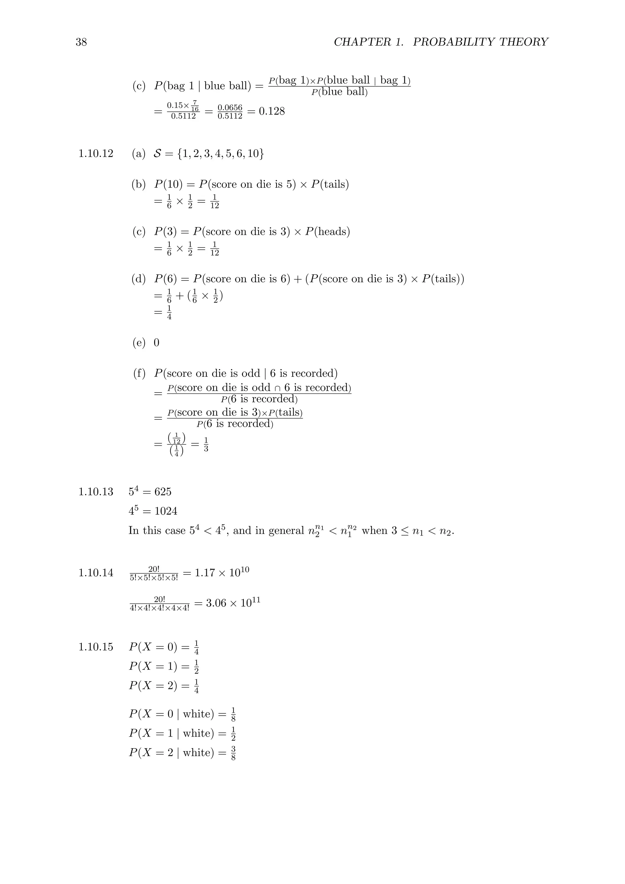
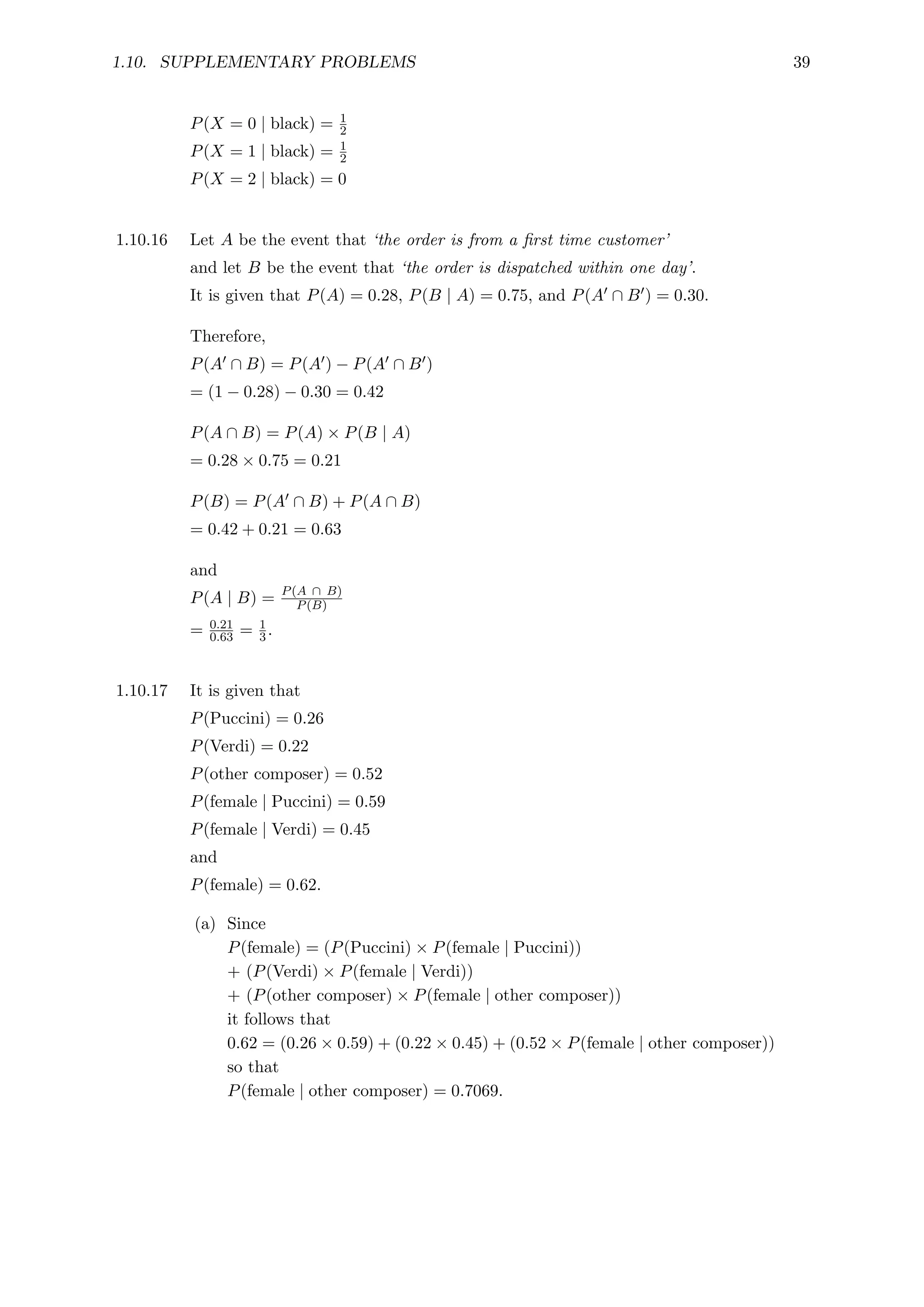
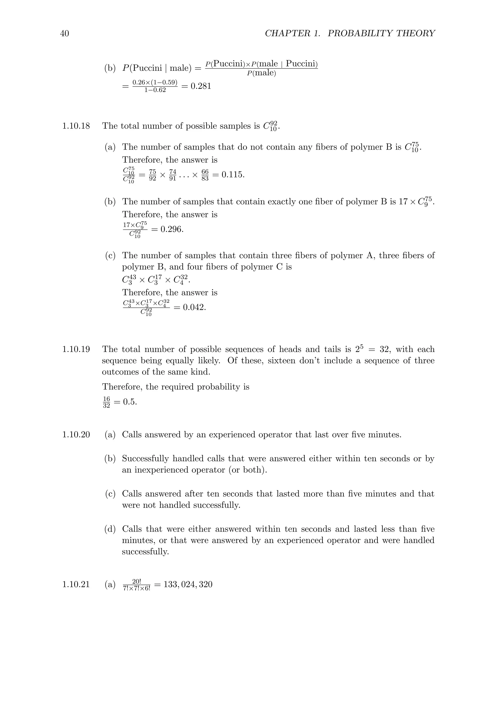
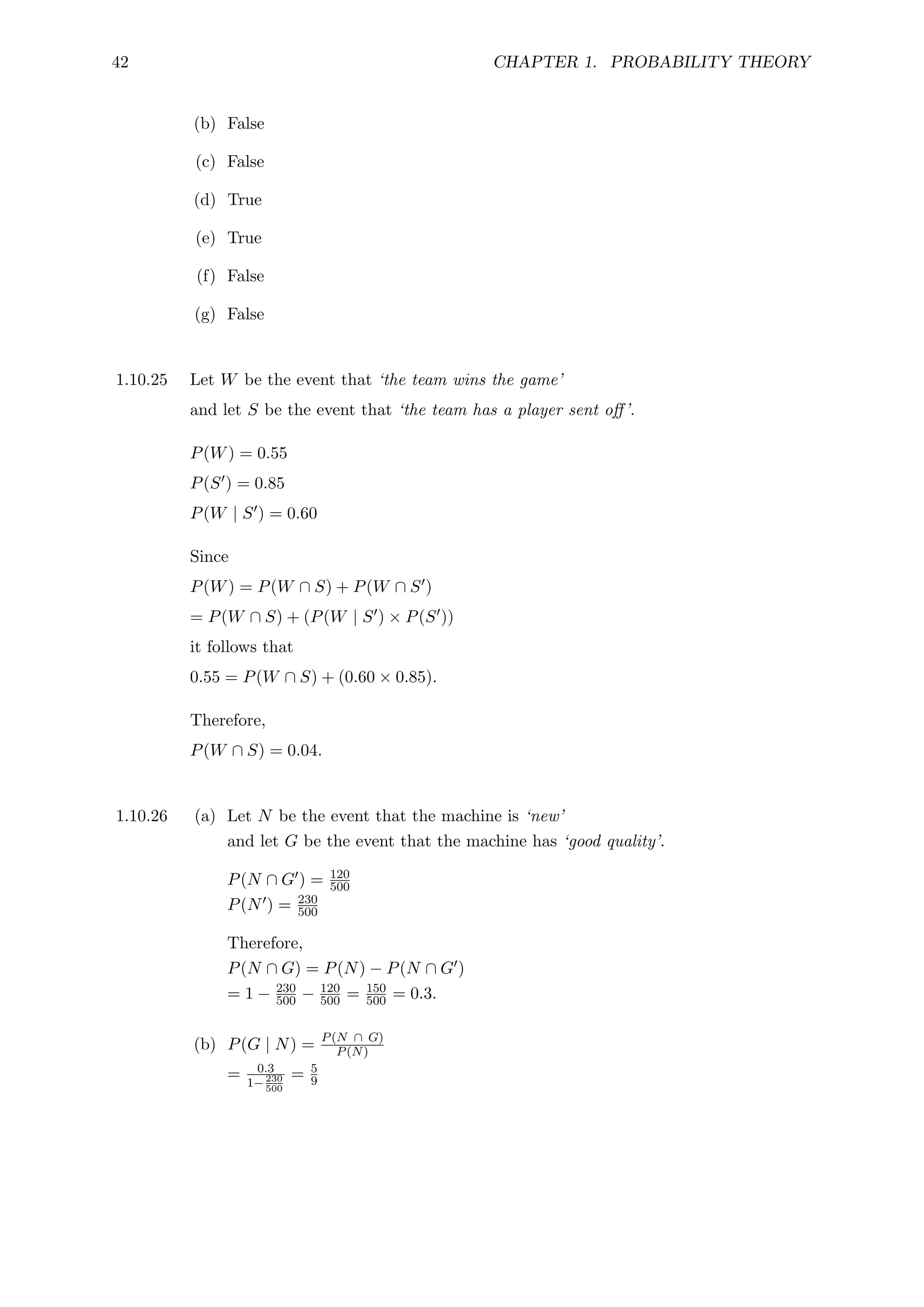
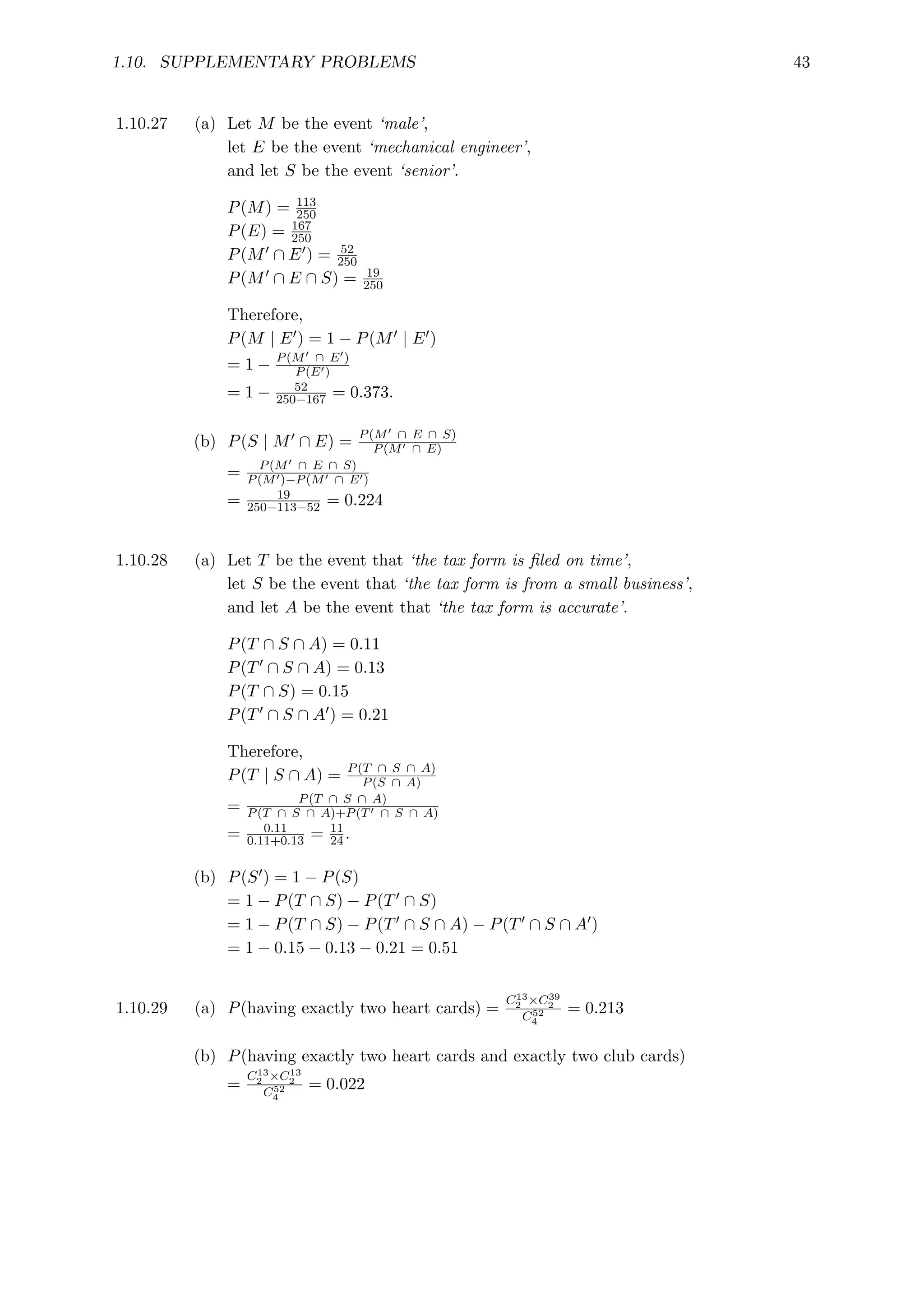
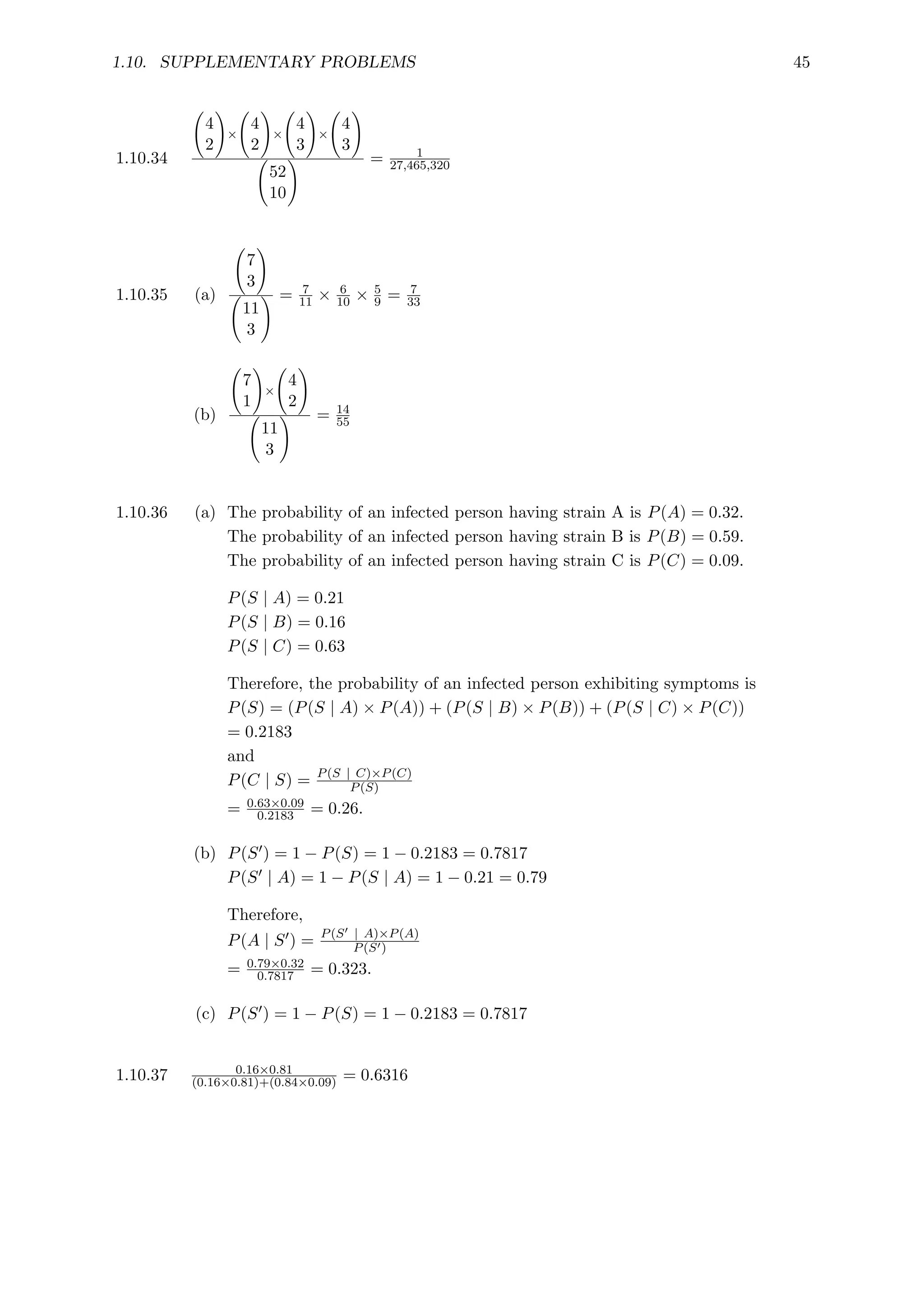
toaz.info-instructor-solution-manual-probability-and-statistics-for-engineers-and-scientis-pr_c34ebffbb22bb7f438f0cfbb63ef4d70.pdf

Instructor Solution Manual
Probability and Statistics for Engineers and Scientists
(4th Edition)
Anthony Hayter

1
Instructor Solution Manual
This instructor solution manual to accompany the fourth edition of
“Probability and Statistics for Engineers and Scientists” by Anthony Hayter
provides worked solutions and answers to almost all of the problems given in the textbook.
The student solution manual provides worked solutions and answers to only the odd-numbered
problems given at the end of the chapter sections. In addition to the material contained in
the student solution manual, this instructor manual therefore provides worked solutions and
answers to the even-numbered problems given at the end of the chapter sections together with
almost all of the supplementary problems at the end of each chapter.

Contents
1 Probability Theory 7
1.1 Probabilities . . . . . . . . . . . . . . . . . . . . . . . . . . . . . . . . . . . . . . . 7
1.2 Events . . . . . . . . . . . . . . . . . . . . . . . . . . . . . . . . . . . . . . . . . . 9
1.3 Combinations of Events . . . . . . . . . . . . . . . . . . . . . . . . . . . . . . . . 12
1.4 Conditional Probability . . . . . . . . . . . . . . . . . . . . . . . . . . . . . . . . 15
1.5 Probabilities of Event Intersections . . . . . . . . . . . . . . . . . . . . . . . . . . 20
1.6 Posterior Probabilities . . . . . . . . . . . . . . . . . . . . . . . . . . . . . . . . . 26
1.7 Counting Techniques . . . . . . . . . . . . . . . . . . . . . . . . . . . . . . . . . . 30
1.10 Supplementary Problems . . . . . . . . . . . . . . . . . . . . . . . . . . . . . . . . 35
2 Random Variables 47
2.1 Discrete Random Variables . . . . . . . . . . . . . . . . . . . . . . . . . . . . . . 47
2.2 Continuous Random Variables . . . . . . . . . . . . . . . . . . . . . . . . . . . . . 52
2.3 The Expectation of a Random Variable . . . . . . . . . . . . . . . . . . . . . . . 56
2.4 The Variance of a Random Variable . . . . . . . . . . . . . . . . . . . . . . . . . 60
2.5 Jointly Distributed Random Variables . . . . . . . . . . . . . . . . . . . . . . . . 66
2.6 Combinations and Functions of Random variables . . . . . . . . . . . . . . . . . . 75
3 Discrete Probability Distributions 93
3.1 The Binomial Distribution . . . . . . . . . . . . . . . . . . . . . . . . . . . . . . . 93
3.2 The Geometric and Negative Binomial Distributions . . . . . . . . . . . . . . . . 97
3.3 The Hypergeometric Distribution . . . . . . . . . . . . . . . . . . . . . . . . . . . 100
3.4 The Poisson Distribution . . . . . . . . . . . . . . . . . . . . . . . . . . . . . . . 103
3.5 The Multinomial Distribution . . . . . . . . . . . . . . . . . . . . . . . . . . . . . 105
4 Continuous Probability Distributions 113
4.1 The Uniform Distribution . . . . . . . . . . . . . . . . . . . . . . . . . . . . . . . 113
4.2 The Exponential Distribution . . . . . . . . . . . . . . . . . . . . . . . . . . . . . 116
4.3 The Gamma Distribution . . . . . . . . . . . . . . . . . . . . . . . . . . . . . . . 119
4.4 The Weibull Distribution . . . . . . . . . . . . . . . . . . . . . . . . . . . . . . . 121
4.5 The Beta Distribution . . . . . . . . . . . . . . . . . . . . . . . . . . . . . . . . . 123
3

4 CONTENTS
5 The Normal Distribution 129
5.1 Probability Calculations using the Normal Distribution . . . . . . . . . . . . . . 129
5.2 Linear Combinations of Normal Random Variables . . . . . . . . . . . . . . . . . 135
5.3 Approximating Distributions with the Normal Distribution . . . . . . . . . . . . 140
5.4 Distributions Related to the Normal Distribution . . . . . . . . . . . . . . . . . . 144
6 Descriptive Statistics 157
6.1 Experimentation . . . . . . . . . . . . . . . . . . . . . . . . . . . . . . . . . . . . 157
6.2 Data Presentation . . . . . . . . . . . . . . . . . . . . . . . . . . . . . . . . . . . 159
6.3 Sample Statistics . . . . . . . . . . . . . . . . . . . . . . . . . . . . . . . . . . . . 161
7 Statistical Estimation and Sampling Distributions 167
7.2 Properties of Point Estimates . . . . . . . . . . . . . . . . . . . . . . . . . . . . . 167
7.3 Sampling Distributions . . . . . . . . . . . . . . . . . . . . . . . . . . . . . . . . . 170
7.4 Constructing Parameter Estimates . . . . . . . . . . . . . . . . . . . . . . . . . . 177
8 Inferences on a Population Mean 185
8.1 Confidence Intervals . . . . . . . . . . . . . . . . . . . . . . . . . . . . . . . . . . 185
8.2 Hypothesis Testing . . . . . . . . . . . . . . . . . . . . . . . . . . . . . . . . . . . 191
9 Comparing Two Population Means 209
9.2 Analysis of Paired Samples . . . . . . . . . . . . . . . . . . . . . . . . . . . . . . 209
9.3 Analysis of Independent Samples . . . . . . . . . . . . . . . . . . . . . . . . . . . 214
10 Discrete Data Analysis 231
10.1 Inferences on a Population Proportion . . . . . . . . . . . . . . . . . . . . . . . . 231
10.2 Comparing Two Population Proportions . . . . . . . . . . . . . . . . . . . . . . . 238
10.3 Goodness of Fit Tests for One-way Contingency Tables . . . . . . . . . . . . . . . 246
10.4 Testing for Independence in Two-way Contingency Tables . . . . . . . . . . . . . 252
11 The Analysis of Variance 269
11.1 One Factor Analysis of Variance . . . . . . . . . . . . . . . . . . . . . . . . . . . 269
11.2 Randomized Block Designs . . . . . . . . . . . . . . . . . . . . . . . . . . . . . . 279
12 Simple Linear Regression and Correlation 293
12.1 The Simple Linear Regression Model . . . . . . . . . . . . . . . . . . . . . . . . . 293
12.2 Fitting the Regression Line . . . . . . . . . . . . . . . . . . . . . . . . . . . . . . 295
12.3 Inferences on the Slope Parameter β̂1 . . . . . . . . . . . . . . . . . . . . . . . . . 298
12.4 Inferences on the Regression Line . . . . . . . . . . . . . . . . . . . . . . . . . . . 302
12.5 Prediction Intervals for Future Response Values . . . . . . . . . . . . . . . . . . . 304
12.6 The Analysis of Variance Table . . . . . . . . . . . . . . . . . . . . . . . . . . . . 306
12.7 Residual Analysis . . . . . . . . . . . . . . . . . . . . . . . . . . . . . . . . . . . . 309

CONTENTS 5
12.8 Variable Transformations . . . . . . . . . . . . . . . . . . . . . . . . . . . . . . . 310
12.9 Correlation Analysis . . . . . . . . . . . . . . . . . . . . . . . . . . . . . . . . . . 312
12.12Supplementary Problems . . . . . . . . . . . . . . . . . . . . . . . . . . . . . . . . 313
13 Multiple Linear Regression and Nonlinear Regression 325
13.1 Introduction to Multiple Linear Regression . . . . . . . . . . . . . . . . . . . . . 325
13.2 Examples of Multiple Linear Regression . . . . . . . . . . . . . . . . . . . . . . . 328
13.3 Matrix Algebra Formulation of Multiple Linear Regression . . . . . . . . . . . . . 330
13.4 Evaluating Model Accuracy . . . . . . . . . . . . . . . . . . . . . . . . . . . . . . 335
14 Multifactor Experimental Design and Analysis 341
14.1 Experiments with Two Factors . . . . . . . . . . . . . . . . . . . . . . . . . . . . 341
14.2 Experiments with Three or More Factors . . . . . . . . . . . . . . . . . . . . . . 344
15 Nonparametric Statistical Analysis 351
15.1 The Analysis of a Single Population . . . . . . . . . . . . . . . . . . . . . . . . . 351
15.2 Comparing Two Populations . . . . . . . . . . . . . . . . . . . . . . . . . . . . . 355
15.3 Comparing Three or More Populations . . . . . . . . . . . . . . . . . . . . . . . . 358
16 Quality Control Methods 367
16.2 Statistical Process Control . . . . . . . . . . . . . . . . . . . . . . . . . . . . . . . 367
16.3 Variable Control Charts . . . . . . . . . . . . . . . . . . . . . . . . . . . . . . . . 369
16.4 Attribute Control Charts . . . . . . . . . . . . . . . . . . . . . . . . . . . . . . . 371
16.5 Acceptance Sampling . . . . . . . . . . . . . . . . . . . . . . . . . . . . . . . . . . 372
17 Reliability Analysis and Life Testing 375
17.1 System Reliability . . . . . . . . . . . . . . . . . . . . . . . . . . . . . . . . . . . 375
17.2 Modeling Failure Rates . . . . . . . . . . . . . . . . . . . . . . . . . . . . . . . . 377
17.3 Life Testing . . . . . . . . . . . . . . . . . . . . . . . . . . . . . . . . . . . . . . . 380

Chapter 1
Probability Theory
1.1 Probabilities
1.1.1 S = {(head, head, head), (head, head, tail), (head, tail, head), (head, tail, tail),
(tail, head, head), (tail, head, tail), (tail, tail, head), (tail, tail, tail)}
1.1.2 S = {0 females, 1 female, 2 females, 3 females, . . . , n females}
1.1.3 S = {0,1,2,3,4}
1.1.4 S = {January 1, January 2, .... , February 29, .... , December 31}
1.1.5 S = {(on time, satisfactory), (on time, unsatisfactory),
(late, satisfactory), (late, unsatisfactory)}
1.1.6 S = {(red, shiny), (red, dull), (blue, shiny), (blue, dull)}
1.1.7 (a) p
1−p = 1 ⇒ p = 0.5
(b) p
1−p = 2 ⇒ p = 2
3
(c) p = 0.25 ⇒ p
1−p = 1
3
1.1.8 0.13 + 0.24 + 0.07 + 0.38 + P(V ) = 1 ⇒ P(V ) = 0.18
7

8 CHAPTER 1. PROBABILITY THEORY
1.1.9 0.08 + 0.20 + 0.33 + P(IV ) + P(V ) = 1 ⇒ P(IV ) + P(V ) = 1 − 0.61 = 0.39
Therefore, 0 ≤ P(V ) ≤ 0.39.
If P(IV ) = P(V ) then P(V ) = 0.195.
1.1.10 P(I) = 2 × P(II) and P(II) = 3 × P(III) ⇒ P(I) = 6 × P(III)
Therefore,
P(I) + P(II) + P(III) = 1
so that
(6 × P(III)) + (3 × P(III)) + P(III) = 1.
Consequently,
P(III) = 1
10, P(II) = 3 × P(III) = 3
10
and
P(I) = 6 × P(III) = 6
10.
1.1.11 p = 1 − 0.28 − 0.55 = 0.17.

1.2. EVENTS 9
1.2 Events
1.2.1 (a) 0.13 + P(b) + 0.48 + 0.02 + 0.22 = 1 ⇒ P(b) = 0.15
(b) A = {c, d} so that P(A) = P(c) + P(d) = 0.48 + 0.02 = 0.50
(c) P(A0) = 1 − P(A) = 1 − 0.5 = 0.50
1.2.2 (a) P(A) = P(b) + P(c) + P(e) = 0.27 so P(b) + 0.11 + 0.06 = 0.27
and hence P(b) = 0.10
(b) P(A0) = 1 − P(A) = 1 − 0.27 = 0.73
(c) P(A0) = P(a) + P(d) + P(f) = 0.73 so 0.09 + P(d) + 0.29 = 0.73
and hence P(d) = 0.35
1.2.3 Over a four year period including one leap year, the number of days is
(3 × 365) + 366 = 1461.
The number of January days is 4 × 31 = 124
and the number of February days is (3 × 28) + 29 = 113.
The answers are therefore 124
1461 and 113
1461.
1.2.4 1 − 0.03 − 0.18 = 0.79
1 − 0.03 = 0.97
1.2.5 1 − 0.38 − 0.11 − 0.16 = 0.35
0.38 + 0.16 + 0.35 = 0.89
1.2.6 In Figure 1.10 let (x, y) represent the outcome that the score on the red die is x and
the score on the blue die is y. The event that the score on the red die is strictly
greater than the score on the blue die consists of the following 15 outcomes:
{(2,1), (3,1), (3,2), (4,1), (4,2), (4,3), (5,1), (5,2), (5,3), (5,4), (6,1), (6,2), (6,3),
(6,4), (6,5)}
The probability of each outcome is 1
36 so the required probability is 15 × 1
36 = 5
12.
This probability is less than 0.5 because of the possibility that both scores are equal.
The complement of this event is the event that the red die has a score less than or
equal to the score on the blue die which has a probability of 1 − 5
12 = 7
12.

1.2.7 P(♠ or ♣) = P(A♠) + P(K♠) + . . . + P(2♠) +P(A♣) + P(K♣) + . . . + P(2♣)
= 1
52 + . . . + 1
52 = 26
52 = 1
2
1.2.8 P(draw an ace) = P(A♠) + P(A♣) + P(A♦) + P(A♥)
= 1
52 + 1
52 + 1
52 + 1
52 = 4
52 = 1
13
1.2.9 (a) Let the four players be named A, B, C, and T for Terica, and let the notation
(X, Y ) indicate that player X is the winner and player Y is the runner up.
The sample space consists of the 12 outcomes:
S = {(A,B), (A,C), (A,T), (B,A), (B,C), (B,T), (C,A), (C,B), (C,T), (T,A),
(T,B), (T,C)}
The event ‘Terica is winner’ consists of the 3 outcomes {(T,A), (T,B), (T,C)}.
Since each outcome in S is equally likely to occur with a probability of 1
12 it
follows that
P(Terica is winner) = 3
12 = 1
4.
(b) The event ‘Terica is winner or runner up’ consists of 6 out of the 12 outcomes
so that
P(Terica is winner or runner up) = 6
12 = 1
2.
1.2.10 (a) See Figure 1.24.
P(Type I battery lasts longest)
= P((II, III, I)) + P((III, II, I))
= 0.39 + 0.03 = 0.42
(b) P(Type I battery lasts shortest)
= P((I, II, III)) + P((I, III, II))
= 0.11 + 0.07 = 0.18
(c) P(Type I battery does not last longest)
= 1 − P(Type I battery lasts longest)
= 1 − 0.42 = 0.58
(d) P(Type I battery last longer than Type II)
= P((II, I, III)) + P((II, III, I)) + P((III, II, I))
= 0.24 + 0.39 + 0.03 = 0.66
1.2.11 (a) See Figure 1.25.
The event ‘both assembly lines are shut down’ consists of the single outcome
{(S,S)}.
Therefore,

1.2. EVENTS 11
P(both assembly lines are shut down) = 0.02.
(b) The event ‘neither assembly line is shut down’ consists of the outcomes
{(P,P), (P,F), (F,P), (F,F)}.
Therefore,
P(neither assembly line is shut down)
= P((P, P)) + P((P, F)) + P((F, P)) + P((F, F))
= 0.14 + 0.2 + 0.21 + 0.19 = 0.74.
(c) The event ‘at least one assembly line is at full capacity’ consists of the outcomes
{(S,F), (P,F), (F,F), (F,S), (F,P)}.
Therefore,
P(at least one assembly line is at full capacity)
= P((S, F)) + P((P, F)) + P((F, F)) + P((F, S)) + P((F, P))
= 0.05 + 0.2 + 0.19 + 0.06 + 0.21 = 0.71.
(d) The event ‘exactly one assembly line at full capacity’ consists of the outcomes
{(S,F), (P,F), (F,S), (F,P)}.
Therefore,
P(exactly one assembly line at full capacity)
= P((S, F)) + P((P, F)) + P((F, S)) + P((F, P))
= 0.05 + 0.20 + 0.06 + 0.21 = 0.52.
The complement of ‘neither assembly line is shut down’ is the event ‘at least one
assembly line is shut down’ which consists of the outcomes
{(S,S), (S,P), (S,F), (P,S), (F,S)}.
The complement of ‘at least one assembly line is at full capacity’ is the event ‘neither
assembly line is at full capacity’ which consists of the outcomes
{(S,S), (S,P), (P,S), (P,P)}.
1.2.12 The sample space is
S = {(H,H,H), (H,T,H), (H,T,T), (H,H,T), (T,H,H), (T,H,T), (T,T,H), (T,T,T)}
with each outcome being equally likely with a probability of 1
8.
The event ‘two heads obtained in succession’ consists of the three outcomes
{(H,H,H), (H,H,T), (T,H,H)}
so that P(two heads in succession) = 3
8.
1.2.13 0.26 + 0.36 + 0.11 = 0.73
1.2.14 0.18 + 0.43 + 0.29 = 0.90

1.3 Combinations of Events
1.3.1 The event A contains the outcome 0 while the empty set does not contain any
outcomes.
1.3.2 (a) See Figure 1.55.
P(B) = 0.01 + 0.02 + 0.05 + 0.11 + 0.08 + 0.06 + 0.13 = 0.46
(b) P(B ∩ C) = 0.02 + 0.05 + 0.11 = 0.18
(c) P(A∪C) = 0.07+0.05+0.01+0.02+0.05+0.08+0.04+0.11+0.07+0.11 = 0.61
(d) P(A ∩ B ∩ C) = 0.02 + 0.05 = 0.07
(e) P(A ∪ B ∪ C) = 1 − 0.03 − 0.04 − 0.05 = 0.88
(f) P(A0 ∩ B) = 0.08 + 0.06 + 0.11 + 0.13 = 0.38
(g) P(B0 ∪ C) = 0.04 + 0.03 + 0.05 + 0.11 + 0.05 + 0.02 + 0.08 + 0.04 + 0.11 + 0.07
+ 0.07 + 0.05 = 0.72
(h) P(A ∪ (B ∩ C)) = 0.07 + 0.05 + 0.01 + 0.02 + 0.05 + 0.08 + 0.04 + 0.11 = 0.43
(i) P((A ∪ B) ∩ C) = 0.11 + 0.05 + 0.02 + 0.08 + 0.04 = 0.30
(j) P(A0 ∪ C) = 0.04 + 0.03 + 0.05 + 0.08 + 0.06 + 0.13 + 0.11 + 0.11 + 0.07 + 0.02
+ 0.05 + 0.08 + 0.04 = 0.87
P(A0 ∪ C)0 = 1 − P(A0 ∪ C) = 1 − 0.87 = 0.13
1.3.4 (a) A ∩ B = {females with black hair}
(b) A ∪ C0 = {all females and any man who does not have brown eyes}
(c) A0 ∩ B ∩ C = {males with black hair and brown eyes}
(d) A ∩ (B ∪ C) = {females with either black hair or brown eyes or both}
1.3.5 Yes, because a card must be drawn from either a red suit or a black suit but it cannot
be from both at the same time.
No, because the ace of hearts could be drawn.

1.3. COMBINATIONS OF EVENTS 13
1.3.6 P(A ∪ B) = P(A) + P(B) − P(A ∩ B) ≤ 1
so that
P(B) ≤ 1 − 0.4 + 0.3 = 0.9.
Also, P(B) ≥ P(A ∩ B) = 0.3
so that
0.3 ≤ P(B) ≤ 0.9.
1.3.7 Since P(A ∪ B) = P(A) + P(B) − P(A ∩ B)
it follows that
P(B) = P(A ∪ B) − P(A) + P(A ∩ B)
= 0.8 − 0.5 + 0.1 = 0.4.
1.3.8 C
1.3.9 Yes, the three events are mutually exclusive because the selected card can only be
from one suit.
Therefore,
P(A ∪ B ∪ C) = P(A) + P(B) + P(C) = 1
4 + 1
4 + 1
4 = 3
4.
A0 is the event ‘a heart is not obtained’ (or similarly the event ‘a club, spade, or
diamond is obtained’ ) so that B is a subset of A0.
1.3.10 (a) A ∩ B = {A♥, A♦}
(b) A ∪ C = {A♥, A♦, A♣, A♠, K♥, K♦, K♣, K♠, Q♥, Q♦, Q♣, Q♠,
J♥, J♦, J♣, J♠}
(c) B ∩ C0 = {A♥, 2♥, . . . , 10♥, A♦, 2♦, . . . , 10♦}
(d) B0 ∩ C = {K♣, K♠, Q♣, Q♠, J♣, J♠}
A ∪ (B0 ∩ C) = {A♥, A♦, A♣, A♠, K♣, K♠, Q♣, Q♠, J♣, J♠}
1.3.11 Let the event O be an on time repair and let the event S be a satisfactory repair.
It is known that P(O ∩ S) = 0.26, P(O) = 0.74 and P(S) = 0.41.
We want to find P(O0 ∩ S0).
Since the event O0 ∩ S0 can be written (O ∪ S)0 it follows that
P(O0 ∩ S0) = 1 − P(O ∪ S)
= 1 − (P(O) + P(S) − P(O ∩ S))

= 1 − (0.74 + 0.41 − 0.26) = 0.11.
1.3.12 Let R be the event that a red ball is chosen and let S be the event that a shiny ball
is chosen.
It is known that P(R ∩ S) = 55
200, P(S) = 91
200 and P(R) = 79
200.
Therefore, the probability that the chosen ball is either shiny or red is
P(R ∪ S) = P(R) + P(S) − P(R ∩ S)
= 79
200 + 91
200 − 55
200
= 115
200 = 0.575.
The probability of a dull blue ball is
P(R0 ∩ S0) = 1 − P(R ∪ S)
= 1 − 0.575 = 0.425.
1.3.13 Let A be the event that the patient is male, let B be the event that the patient is
younger than thirty years of age, and let C be the event that the patient is admitted
to the hospital.
It is given that P(A) = 0.45, P(B) = 0.30, P(A0 ∩ B0 ∩ C) = 0.15,
and P(A0 ∩ B) = 0.21.
The question asks for P(A0 ∩ B0 ∩ C0).
Notice that
P(A0 ∩ B0) = P(A0) − P(A0 ∩ B) = (1 − 0.45) − 0.21 = 0.34
so that
P(A0 ∩ B0 ∩ C0) = P(A0 ∩ B0) − P(A0 ∩ B0 ∩ C) = 0.34 − 0.15 = 0.19.
1.3.14 P(A ∩ B) = 0.26
P(A ∪ B) = 1
1.3.15 P(A ∩ B) = P(B) = 0.43 + 0.29 = 0.72
P(A ∪ B) = P(A) = 0.18 + 0.43 + 0.29 = 0.90

1.4. CONDITIONAL PROBABILITY 15
1.4 Conditional Probability
1.4.1 See Figure 1.55.
(a) P(A | B) = P(A∩B)
P(B) = 0.02+0.05+0.01
0.02+0.05+0.01+0.11+0.08+0.06+0.13 = 0.1739
(b) P(C | A) = P(A∩C)
P(A) = 0.02+0.05+0.08+0.04
0.02+0.05+0.08+0.04+0.018+0.07+0.05 = 0.59375
(c) P(B | A ∩ B) = P(B∩(A∩B))
P(A∩B) = P(A∩B)
P(A∩B) = 1
(d) P(B | A ∪ B) = P(B∩(A∪B))
P(A∪B) = P(B)
P(A∪B) = 0.46
0.46+0.32−0.08 = 0.657
(e) P(A | A ∪ B ∪ C) = P(A∩(A∪B∪C))
P(A∪B∪C) = P(A)
P(A∪B∪C) = 0.32
1−0.04−0.05−0.03 = 0.3636
(f) P(A ∩ B | A ∪ B) = P((A∩B)∩(A∪B))
P(A∪B) = P(A∩B)
P(A∪B) = 0.08
0.7 = 0.1143
1.4.2 (a) 0.42 × 0.42 × 0.42 = 0.0741
(b) 0.42 × (1 − 0.63) = 0.1554
1.4.3 (a) P(A♥ | red suit) = P(A♥∩red suit)
P(red suit)
= P(A♥)
P(red suit)
=
( 1
52 )
(26
52 )
= 1
26
(b) P(heart | red suit) = P(heart∩red suit)
P(red suit)
= P(heart)
P(red suit)
=
(13
52 )
(26
52 )
= 13
26 = 1
2
(c) P(red suit | heart) = P(red suit∩heart)
P(heart)
= P(heart)
P(heart)
= 1
(d) P(heart | black suit) = P(heart∩black suit)
P(black suit)
= P(∅)
P(black suit)
= 0
(e) P(King | red suit) = P(King∩red suit)
P(red suit)
= P(K♥, K♦)
P(red suit)
=
( 2
52 )
(26
52 )
= 2
26 = 1
13
(f) P(King | red picture card) = P(King∩red picture card)
P(red picture card)
= P(K♥, K♦)
P(red picture card)
=
( 2
52 )
( 6
52 )
= 2
6 = 1
3
1.4.4 P(A) is smaller than P(A | B).
Event B is a necessary condition for event A and so conditioning on event B increases
the probability of event A.

1.4.5 There are 54 blue balls and so there are 150 − 54 = 96 red balls.
Also, there are 36 shiny, red balls and so there are 96 − 36 = 60 dull, red balls.
P(shiny | red) = P(shiny ∩ red)
P(red)
=
( 36
150 )
( 96
150 )
= 36
96 = 3
8
P(dull | red) = P(dull ∩ red)
P(red)
=
( 60
150 )
( 96
150 )
= 60
96 = 5
8
1.4.6 Let the event O be an on time repair and let the event S be a satisfactory repair.
It is known that P(S | O) = 0.85 and P(O) = 0.77.
The question asks for P(O ∩ S) which is
P(O ∩ S) = P(S | O) × P(O) = 0.85 × 0.77 = 0.6545.
1.4.7 (a) It depends on the weather patterns in the particular location that is being
considered.
(b) It increases since there are proportionally more black haired people among
brown eyed people than there are in the general population.
(c) It remains unchanged.
(d) It increases.
1.4.8 Over a four year period including one leap year the total number of days is
(3 × 365) + 366 = 1461.
Of these, 4 × 12 = 48 days occur on the first day of a month and so the probability
that a birthday falls on the first day of a month is
48
1461 = 0.0329.
Also, 4 × 31 = 124 days occur in March of which 4 days are March 1st.
Consequently, the probability that a birthday falls on March 1st. conditional that it
is in March is
4
124 = 1
31 = 0.0323.
Finally, (3×28)+29 = 113 days occur in February of which 4 days are February 1st.
Consequently, the probability that a birthday falls on February 1st. conditional that
it is in February is
4
113 = 0.0354.

1.4.9 (a) Let A be the event that ‘Type I battery lasts longest’ consisting of the outcomes
{(III, II, I), (II, III, I)}.
Let B be the event that ‘Type I battery does not fail first’ consisting of the
outcomes {(III,II,I), (II,III,I), (II,I,III), (III,I,II)}.
The event A ∩ B = {(III,II,I), (II,III,I)} is the same as event A.
Therefore,
P(A | B) = P(A∩B)
P(B) = 0.39+0.03
0.39+0.03+0.24+0.16 = 0.512.
(b) Let C be the event that ‘Type II battery fails first’ consisting of the outcomes
{(II,I,III), (II,III,I)}.
Thus, A ∩ C = {(II, III, I)} and therefore
P(A | C) = P(A∩C)
P(C) = 0.39
0.39+0.24 = 0.619.
(c) Let D be the event that ‘Type II battery lasts longest’ consisting of the outcomes
{(I,III,II), (III,I,II)}.
Thus, A ∩ D = ∅ and therefore
P(A | D) = P(A∩D)
P(D) = 0.
(d) Let E be the event that ‘Type II battery does not fail first’ consisting of the
outcomes {(I,III,II), (I,II,III), (III,II,I), (III,I,II)}.
Thus, A ∩ E = {(III, II, I)} and therefore
P(A | E) = P(A∩E)
P(E) = 0.03
0.07+0.11+0.03+0.16 = 0.081.
1.4.10 See Figure 1.25.
(a) Let A be the event ‘both lines at full capacity’ consisting of the outcome {(F,F)}.
Let B be the event ‘neither line is shut down’ consisting of the outcomes
{(P,P), (P,F), (F,P), (F,F)}.
Thus, A ∩ B = {(F, F)} and therefore
P(A | B) = P(A∩B)
P(B) = 0.19
(0.14+0.2+0.21+0.19) = 0.257.
(b) Let C be the event ‘at least one line at full capacity’ consisting of the outcomes
{(F,P), (F,S), (F,F), (S,F), (P,F)}.
Thus, C ∩ B = {(F, P), (F, F), (P, F)} and therefore
P(C | B) = P(C∩B)
P(B) = 0.21+0.19+0.2
0.74 = 0.811.
(c) Let D be the event that ‘one line is at full capacity’ consisting of the outcomes
{(F,P), (F,S), (P,F), (S,F)}.
Let E be the event ‘one line is shut down’ consisting of the outcomes
{(S,P), (S,F), (P,S), (F,S)}.
Thus, D ∩ E = {(F, S), (S, F)} and therefore
P(D | E) = P(D∩E)
P(E) = 0.06+0.05
0.06+0.05+0.07+0.06 = 0.458.

(d) Let G be the event that ‘neither line is at full capacity’ consisting of the
outcomes {(S,S), (S,P), (P,S), (P,P)}.
Let H be the event that ‘at least one line is at partial capacity’ consisting of
the outcomes {(S,P), (P,S), (P,P), (P,F), (F,P)}.
Thus, F ∩ G = {(S, P), (P, S), (P, P)} and therefore
P(F | G) = P(F∩G)
P(G) = 0.06+0.07+0.14
0.06+0.07+0.14+0.2+0.21 = 0.397.
1.4.11 Let L, W and H be the events that the length, width and height respectively are
within the specified tolerance limits.
It is given that P(W) = 0.86, P(L ∩ W ∩ H) = 0.80, P(L ∩ W ∩ H0) = 0.02,
P(L0 ∩ W ∩ H) = 0.03 and P(W ∪ H) = 0.92.
(a) P(W ∩ H) = P(L ∩ W ∩ H) + P(L0 ∩ W ∩ H) = 0.80 + 0.03 = 0.83
P(H) = P(W ∪ H) − P(W) + P(W ∩ H) = 0.92 − 0.86 + 0.83 = 0.89
P(W ∩ H | H) = P(W∩H)
P(H) = 0.83
0.89 = 0.9326
(b) P(L ∩ W) = P(L ∩ W ∩ H) + P(L ∩ W ∩ H0) = 0.80 + 0.02 = 0.82
P(L ∩ W ∩ H | L ∩ W) = P(L ∩ W ∩ H)
P(L ∩ W) = 0.80
0.82 = 0.9756
1.4.12 Let A be the event that the gene is of ‘type A’, and let D be the event that the gene
is ‘dominant’.
P(D | A0) = 0.31
P(A0 ∩ D) = 0.22
Therefore,
P(A) = 1 − P(A0)
= 1 − P(A0∩D)
P(D|A0)
= 1 − 0.22
0.31 = 0.290
1.4.13 (a) Let E be the event that the ‘component passes on performance’, let A be the
event that the ‘component passes on appearance’, and let C be the event that
the ‘component passes on cost’.
P(A ∩ C) = 0.40
P(E ∩ A ∩ C) = 0.31
P(E) = 0.64
P(E0 ∩ A0 ∩ C0) = 0.19
P(E0 ∩ A ∩ C0) = 0.06
Therefore,
P(E0 ∩ A0 ∩ C) = P(E0 ∩ A0) − P(E0 ∩ A0 ∩ C0)
= P(E0) − P(E0 ∩ A) − 0.19

= 1 − P(E) − P(E0 ∩ A ∩ C) − P(E0 ∩ A ∩ C0) − 0.19
= 1 − 0.64 − P(A ∩ C) + P(E ∩ A ∩ C) − 0.06 − 0.19
= 1 − 0.64 − 0.40 + 0.31 − 0.06 − 0.19 = 0.02
(b) P(E ∩ A ∩ C | A ∩ C) = P(E∩A∩C)
P(A∩C)
= 0.31
0.40 = 0.775
1.4.14 (a) Let T be the event ‘good taste’, let S be the event ‘good size’, and let A be the
event ‘good appearance’.
P(T) = 0.78
P(T ∩ S) = 0.69
P(T ∩ S0 ∩ A) = 0.05
P(S ∪ A) = 0.84
Therefore,
P(S | T) = P(T∩S)
P(T) = 0.69
0.78 = 0.885.
(b) Notice that
P(S0 ∩ A0) = 1 − P(S ∪ A) = 1 − 0.84 = 0.16.
Also,
P(T ∩ S0) = P(T) − P(T ∩ S) = 0.78 − 0.69 = 0.09
so that
P(T ∩ S0 ∩ A0) = P(T ∩ S0) − P(T ∩ S0 ∩ A) = 0.09 − 0.05 = 0.04.
Therefore,
P(T | S0 ∩ A0) = P(T∩S0∩A0)
P(S0∩A0) = 0.04
0.16 = 0.25.
1.4.15 P(delay) = (P(delay | technical problems) × P(technical problems))
+ (P(delay | no technical problems) × P(no technical problems))
= (1 × 0.04) + (0.33 × 0.96) = 0.3568
1.4.16 Let S be the event that a chip ‘survives 500 temperature cycles’ and let A be the
event that the chip was ‘made by company A’.
P(S) = 0.42
P(A | S0) = 0.73
Therefore,
P(A0 ∩ S0) = P(S0) × P(A0 | S0) = (1 − 0.42) × (1 − 0.73) = 0.1566.
1.4.17 0.26
0.26+0.36+0.11 = 0.3562
1.4.18 0.43+0.29
0.18+0.43+0.29 = 0.8

1.5 Probabilities of Event Intersections
1.5.1 (a) P(both cards are picture cards) = 12
52 × 11
51 = 132
2652
(b) P(both cards are from red suits) = 26
52 × 25
51 = 650
2652
(c) P(one card is from a red suit and one is from black suit)
= (P(first card is red) × P(2nd card is black | 1st card is red))
+ (P(first card is black) × P(2nd card is red | 1st card is black))
=

26
52 × 26
51

+

26
52 × 26
51

= 676
2652 × 2 = 26
51
1.5.2 (a) P(both cards are picture cards) = 12
52 × 12
52 = 9
169
The probability increases with replacement.
(b) P(both cards are from red suits) = 26
52 × 26
52 = 1
4
(c) P(one card is from a red suit and one is from black suit)
= (P(first card is red) × P(2nd card is black | 1st card is red))
+ (P(first card is black) × P(2nd card is red | 1st card is black))
=

26
52 × 26
52

+

26
52 × 26
52

= 1
2
The probability decreases with replacement.
1.5.3 (a) No, they are not independent.
Notice that
P((ii)) = 3
13 6= P((ii) | (i)) = 11
51.
(b) Yes, they are independent.
Notice that
P((i) ∩ (ii)) = P((i)) × P((ii))
since
P((i)) = 1
4
P((ii)) = 3
13
and
P((i) ∩ (ii)) = P(first card a heart picture ∩ (ii))
+ P(first card a heart but not a picture ∩ (ii))
=

3
52 × 11
51

+

10
52 × 12
51

= 153
2652 = 3
52.
(c) No, they are not independent.
Notice that
P((ii)) = 1
2 6= P((ii) | (i)) = 25
51.

1.5. PROBABILITIES OF EVENT INTERSECTIONS 21
(d) Yes, they are independent.
Similar to part (b).
(e) No, they are not independent.
1.5.4 P(all four cards are hearts) = P(lst card is a heart)
×P(2nd card is a heart | lst card is a heart)
×P(3rd card is a heart | 1st and 2nd cards are hearts)
×P(4th card is a heart | 1st, 2nd and 3rd cards are hearts)
= 13
52 × 12
51 × 11
50 × 10
49 = 0.00264
P(all 4 cards from red suits) = P(1st card from red suit)
×P(2nd card is from red suit | lst card is from red suit)
×P(3rd card is from red suit | 1st and 2nd cards are from red suits)
×P(4th card is from red suit | 1st, 2nd and 3rd cards are from red suits)
= 26
52 × 25
51 × 24
50 × 23
49 = 0.055
P(all 4 cards from different suits) = P(1st card from any suit)
×P(2nd card not from suit of 1st card)
×P(3rd card not from suit of 1st or 2nd cards)
×P(4th card not from suit of 1st, 2nd, or 3rd cards)
= 1 × 39
51 × 26
50 × 13
49 = 0.105
1.5.5 P(all 4 cards are hearts) = (13
52)4 = 1
256
P(all 4 cards are from red suits) = (26
52)4 = 1
16
P(all 4 cards from different suits) = 1 × 39
52 × 26
52 × 13
52 = 3
32
The probability decreases with replacement.
1.5.6 The events A and B are independent so that P(A | B) = P(A), P(B | A) = P(B),
and P(A ∩ B) = P(A)P(B).
To show that two events are independent it needs to be shown that one of the above
three conditions holds.
(a) Recall that
P(A ∩ B) + P(A ∩ B0) = P(A)
and

P(B) + P(B0) = 1.
Therefore,
P(A | B0) = P(A∩B0)
P(B0)
= P(A)−P(A∩B)
1−P(B)
= P(A)−P(A)P(B)
1−P(B)
= P(A)(1−P(B))
1−P(B)
= P(A).
(b) Similar to part (a).
(c) P(A0 ∩ B0) + P(A0 ∩ B) = P(A0)
so that
P(A0 ∩ B0) = P(A) − P(A0 ∩ B) = P(A) − P(A0)P(B)
since the events A0 and B are independent.
Therefore,
P(A0 ∩ B0) = P(A)(1 − P(B)) = P(A0)P(B0).
1.5.7 The only way that a message will not get through the network is if both branches are
closed at the same time. The branches are independent since the switches operate
independently of each other.
Therefore,
P(message gets through the network)
= 1 − P(message cannot get through the top branch or the bottom branch)
= 1 − (P(message cannot get through the top branch)
× P(message cannot get through the bottom branch)).
Also,
P(message gets through the top branch) = P(switch 1 is open ∩ switch 2 is open)
= P(switch 1 is open) × P(switch 2 is open)
= 0.88 × 0.92 = 0.8096
since the switches operate independently of each other.
Therefore,
P(message cannot get through the top branch)
= 1 − P(message gets through the top branch)
= 1 − 0.8096 = 0.1904.
Furthermore,
P(message cannot get through the bottom branch)

= P(switch 3 is closed) = 1 − 0.9 = 0.1.
Therefore,
P(message gets through the network) = 1 − (0.1 × 0.1904) = 0.98096.
1.5.8 Given the birthday of the first person, the second person has a different birthday
with a probability 364
365.
The third person has a different birthday from the first two people with a probability
363
365, and so the probability that all three people have different birthdays is
1 × 364
365 × 363
365.
Continuing in this manner the probability that n people all have different birthdays
is therefore
364
365 × 363
365 × 362
365 × . . . × 366−n
365
and
P(at least 2 people out of n share the same birthday)
= 1 − P(n people all have different birthdays)
= 1 −

364
365 × 363
365 × . . . 366−n
365

.
This probability is equal to 0.117 for n = 10,
is equal to 0.253 for n = 15,
and is equal to 0.814 for n = 35.
The smallest values of n for which the probability is greater than 0.5 is n = 23.
Note that in these calculations it has been assumed that birthdays are equally likely
to occur on any day of the year, although in practice seasonal variations may be
observed in the number of births.
1.5.9 P(no broken bulbs) = 83
100 × 82
99 × 81
98 = 0.5682
P(one broken bulb) = P(broken, not broken, not broken)
+ P(not broken, broken, not broken) + P(not broken, not broken, broken)
=

17
100 × 83
99 × 82
98

+

83
100 × 17
99 × 82
98

+

83
100 × 82
99 × 17
98

= 0.3578
P(no more than one broken bulb in the sample)
= P(no broken bulbs) + P(one broken bulb)
= 0.5682 + 0.3578 = 0.9260

1.5.10 P(no broken bulbs) = 83
100 × 83
100 × 83
100 = 0.5718
P(one broken bulb) = P(broken, not broken, not broken)
+ P(not broken, broken, not broken) + P(not broken, not broken, broken)
=

17
100 × 83
100 × 83
100

+

83
100 × 17
100 × 83
100

+

83
100 × 83
100 × 17
100

= 0.3513
P(no more than one broken bulb in the sample)
= P(no broken bulbs) + P(one broken bulb)
= 0.5718 + 0.3513 = 0.9231
The probability of finding no broken bulbs increases with replacement, but the prob-
ability of finding no more than one broken bulb decreases with replacement.
1.5.11 P(drawing 2 green balls)
= P(1st ball is green) × P(2nd ball is green | 1st ball is green)
= 72
169 × 71
168 = 0.180
P(two balls same color)
= P(two red balls) + P(two blue balls) + P(two green balls)
=

43
169 × 42
168

+

54
169 × 53
168

+

72
169 × 71
168

= 0.344
P(two balls different colors) = 1 − P(two balls same color)
= 1 − 0.344 = 0.656
1.5.12 P(drawing 2 green balls) = 72
169 × 72
169 = 0.182
P(two balls same color)
= P(two red balls) + P(two blue balls) + P(two green balls)
=

43
169 × 43
169

+

54
169 × 54
169

+

72
169 × 72
169

= 0.348
P(two balls different colors) = 1 − P(two balls same color)
= 1 − 0.348 = 0.652
The probability that the two balls are green increases with replacement while the
probability of drawing two balls of different colors decreases with replacement.
1.5.13 P(same result on both throws) = P(both heads) + P(both tails)
= p2 + (1 − p)2 = 2p2 − 2p + 1 = 2(p − 0.5)2 + 0.5
which is minimized when p = 0.5 (a fair coin).

1.5.14 P(each score is obtained exactly once)
= 1 × 5
6 × 4
6 × 3
6 × 2
6 × 1
6 = 5
324
P(no sixes in seven rolls) =

5
6
7
= 0.279
1.5.15 (a)

1
2
5
= 1
32
(b) 1 × 5
6 × 4
6 = 5
9
(c) P(BBR) + P(BRB) + P(RBB)
=

1
2 × 1
2 × 1
2

+

1
2 × 1
2 × 1
2

+

1
2 × 1
2 × 1
2

= 3
8
(d) P(BBR) + P(BRB) + P(RBB)
=

26
52 × 25
51 × 26
50

+

26
52 × 26
51 × 25
50

+

26
52 × 26
51 × 25
50

= 13
34
1.5.16 1 − (1 − 0.90)n ≥ 0.995
is satisfied for n ≥ 3.
1.5.17 Claims from clients in the same geographical area would not be independent of each
other since they would all be affected by the same flooding events.
1.5.18 (a) P(system works) = 0.88 × 0.78 × 0.92 × 0.85 = 0.537
(b) P(system works) = 1 − P(no computers working)
= 1 − ((1 − 0.88) × (1 − 0.78) × (1 − 0.92) × (1 − 0.85)) = 0.9997
(c) P(system works) = P(all computers working)
+ P(computers 1,2,3 working, computer 4 not working)
= 0.537 + (0.88 × 0.78 × 0.92 × (1 − 0.85)) + (0.88 × 0.78 × (1 − 0.92) × 0.85)
+ (0.88 × (1 − 0.78) × 0.92 × 0.85) + ((1 − 0.88) × 0.78 × 0.92 × 0.85)
= 0.903
1.5.19 (0.26 + 0.36 + 0.11) × (0.26 + 0.36 + 0.11) = 0.5329
1.5.20 (0.43 + 0.29) × (0.43 + 0.29) × (0.43 + 0.29) × (0.43 + 0.29) = 0.2687

1.6 Posterior Probabilities
1.6.1 (a) The following information is given:
P(disease) = 0.01
P(no disease) = 0.99
P(positive blood test | disease) = 0.97
P(positive blood test | no disease) = 0.06
Therefore,
P(positive blood test) = (P(positive blood test | disease) × P(disease))
+ (P(positive blood test | no disease) × P(no disease))
= (0.97 × 0.01) + (0.06 × 0.99) = 0.0691.
(b) P(disease | positive blood test)
= P(positive blood test ∩ disease)
P(positive blood test)
= P(positive blood test | disease)×P(disease)
P(positive blood test)
= 0.97×0.01
0.0691 = 0.1404
(c) P(no disease | negative blood test)
= P(no disease ∩ negative blood test)
P(negative blood test)
= P(negative blood test | no disease)×P(no disease)
1−P(positive blood test)
= (1−0.06)×0.99
(1−0.0691) = 0.9997
1.6.2 (a) P(red) = (P(red | bag 1) × P(bag 1)) + (P(red | bag 2) × P(bag 2))
+ (P(red | bag 3) × P(bag 3))
=

1
3 × 3
10

+

1
3 × 8
12

+

1
3 × 5
16

= 0.426
(b) P(blue) = 1 − P(red) = 1 − 0.426 = 0.574
(c) P(red ball from bag 2) = P(bag 2) × P(red ball | bag 2)
= 1
3 × 8
12 = 2
9
P(bag 1 | red ball) = P(bag 1 ∩ red ball)
P(red ball)
= P(bag 1)×P(red ball | bag 1)
P(red ball)
=
1
3
× 3
10
0.426 = 0.235
P(bag 2 | blue ball) = P(bag 2 ∩ blue ball)
P(blue ball)
= P(bag 2)×P(blue ball | bag 1)
P(blue ball)

1.6. POSTERIOR PROBABILITIES 27
=
1
3
× 4
12
0.574 = 0.194
1.6.3 (a) P(Section I) = 55
100
(b) P(grade is A)
= (P(A | Section I) × P(Section I)) + (P(A | Section II) × P(Section II))
=

10
55 × 55
100

+

11
45 × 45
100

= 21
100
(c) P(A | Section I) = 10
55
(d) P(Section I | A) = P(A ∩ Section I)
P(A)
= P(Section I)×P(A | Section I)
P(A)
=
55
100
×10
55
21
100
= 10
21
1.6.4 The following information is given:
P(Species 1) = 0.45
P(Species 2) = 0.38
P(Species 3) = 0.17
P(Tagged | Species 1) = 0.10
Therefore,
P(Tagged) = (P(Tagged | Species 1) × P(Species 1))
+ (P(Tagged | Species 2) × P(Species 2)) + (P(Tagged | Species 3) × P(Species 3))
= (0.10 × 0.45) + (0.15 × 0.38) + (0.50 × 0.17) = 0.187.
P(Species 1 | Tagged) = P(Tagged ∩ Species 1)
P(Tagged)
= P(Species 1)×P(Tagged | Species 1)
P(Tagged)
= 0.45×0.10
0.187 = 0.2406
P(Tagged)
P(Tagged)
= 0.38×0.15
0.187 = 0.3048
P(Tagged)

1.7 Counting Techniques
1.7.1 (a) 7! = 7 × 6 × 5 × 4 × 3 × 2 × 1 = 5040
(b) 8! = 8 × 7! = 40320
(c) 4! = 4 × 3 × 2 × 1 = 24
(d) 13! = 13 × 12 × 11 × . . . × 1 = 6,227,020,800
1.7.2 (a) P7
2 = 7!
(7−2)! = 7 × 6 = 42
(b) P9
5 = 9!
(9−5)! = 9 × 8 × 7 × 6 × 5 = 15120
(c) P5
2 = 5!
(5−2)! = 5 × 4 = 20
(d) P17
4 = 17!
(17−4)! = 17 × 16 × 15 × 14 = 57120
1.7.3 (a) C6
2 = 6!
(6−2)!×2! = 6×5
2 = 15
(b) C8
4 = 8!
(8−4)!×4! = 8×7×6×5
24 = 70
(c) C5
2 = 5!
(5−2)!×2! = 5×4
2 = 10
(d) C14
6 = 14!
(14−6)!×6! = 3003
1.7.4 The number of full meals is 5 × 3 × 7 × 6 × 8 = 5040.
The number of meals with just soup or appetizer is (5 + 3) × 7 × 6 × 8 = 2688.
1.7.5 The number of experimental configurations is 3 × 4 × 2 = 24.
1.7.6 (a) Let the notation (2,3,1,4) represent the result that the player who finished 1st
in tournament 1 finished 2nd in tournament 2, the player who finished 2nd
in tournament 1 finished 3rd in tournament 2, the player who finished 3rd in
tournament 1 finished 1st in tournament 2, and the player who finished 4th in
tournament 1 finished 4th in tournament 2.
Then the result (1,2,3,4) indicates that each competitor received the same rank-
ing in both tournaments.

1.7. COUNTING TECHNIQUES 31
Altogether there are 4! = 24 different results, each equally likely, and so this
single result has a probability of 1
24.
(b) The results where no player receives the same ranking in the two tournaments
are:
(2,1,4,3), (2,3,4,1), (2,4,1,3), (3,1,4,2), (3,4,1,2) (3,4,2,1), (4,1,2,3), (4,3,1,2),
(4,3,2,1)
There are nine of these results and so the required probability is 9
24 = 3
8.
1.7.7 The number of rankings that can be assigned to the top 5 competitors is
P20
5 = 20!
15! = 20 × 19 × 18 × 17 × 16 = 1,860,480.
The number of ways in which the best 5 competitors can be chosen is
C20
5 = 20!
15!×5! = 15504.
1.7.8 (a) C100
3 = 100!
97!×3! = 100×99×98
6 = 161700
(b) C83
3 = 83!
80!×3! = 83×82×81
6 = 91881
(c) P(no broken lightbulbs) = 91881
161700 = 0.568
(d) 17 × C83
2 = 17 × 83×82
2 = 57851
(e) The number of samples with 0 or 1 broken bulbs is
91881 + 57851 = 149732.
P(sample contains no more than 1 broken bulb) = 149732
161700 = 0.926
1.7.9 Cn−1
k + Cn−1
k−1 = (n−1)!
k!(n−1−k)! + (n−1)!
(k−1)!(n−k)! = n!
k!(n−k)!

n−k
n + k
n

= n!
k!(n−k)! = Cn
k
This relationship can be interpreted in the following manner.
Cn
k is the number of ways that k balls can be selected from n balls. Suppose that
one ball is red while the remaining n − 1 balls are blue. Either all k balls selected
are blue or one of the selected balls is red. Cn−1
k is the number of ways k blue balls
can be selected while Cn−1
k−1 is the number of ways of selecting the one red ball and
k − 1 blue balls.
1.7.10 (a) The number of possible 5 card hands is C52
5 = 52!
47!×5! =2,598,960.
(b) The number of ways to get a hand of 5 hearts is C13
5 = 13!
8!×5! = 1287.
(c) The number of ways to get a flush is 4 × C13
5 = 4 × 1, 287 = 5148.

(d) P(flush) = 5148
2,598,960 = 0.00198.
(e) There are 48 choices for the fifth card in the hand and so the number of hands
containing all four aces is 48.
(f) 13 × 48 = 624
(g) P(hand has four cards of the same number or picture) = 624
2,598,960 = 0.00024.
1.7.11 There are n! ways in which n objects can be arranged in a line. If the line is made
into a circle and rotations of the circle are considered to be indistinguishable, then
there are n arrangements of the line corresponding to each arrangement of the circle.
Consequently, there are n!
n = (n − 1)! ways to order the objects in a circle.
1.7.12 The number of ways that six people can sit in a line at a cinema is 6! = 720.
See the previous problem.
The number of ways that six people can sit around a dinner table is 5! = 120.
1.7.13 Consider 5 blocks, one block being Andrea and Scott and the other four blocks being
the other four people. At the cinema these 5 blocks can be arranged in 5! ways, and
then Andrea and Scott can be arranged in two different ways within their block, so
that the total number of seating arrangements is 2 × 5! = 240.
Similarly, the total number of seating arrangements at the dinner table is 2×4! = 48.
If Andrea refuses to sit next to Scott then the number of seating arrangements can
be obtained by subtraction. The total number of seating arrangements at the cinema
is 720 − 240 = 480 and the total number of seating arrangements at the dinner table
is 120 − 48 = 72.
1.7.14 The total number of arrangements of n balls is n! which needs to be divided by n1!
because the rearrangements of the n1 balls in box 1 are indistinguishable, and simi-
larly it needs to be divided by n2! . . . nk! due to the indistinguishable rearrangements
possible in boxes 2 to k.
When k = 2 the problem is equivalent to the number of ways of selecting n1 balls
(or n2 balls) from n = n1 + n2 balls.
1.7.15 (a) Using the result provided in the previous problem the answer is 12!
3!×4!×5! = 27720.
(b) Suppose that the balls in part (a) are labelled from 1 to 12. Then the positions
of the three red balls in the line (where the places in the line are labelled 1 to

1.7. COUNTING TECHNIQUES 33
12) can denote which balls in part (a) are placed in the first box, the positions
of the four blue balls in the line can denote which balls in part (a) are placed in
the second box, and the positions of the five green balls in the line can denote
which balls in part (a) are placed in the third box. Thus, there is a one-to-one
correspondence between the positioning of the colored balls in part (b) and the
arrangements of the balls in part (a) so that the problems are identical.
1.7.16 14!
3!×4!×7! = 120120
1.7.17 15!
3!×3!×3!×3!×3! = 168,168,000
1.7.18 The total number of possible samples is C60
12 .
(a) The number of samples containing only items which have either excellent or
good quality is C43
12 .
Therefore, the answer is
C43
12
C60
12
= 43
60 × 42
59 . . . × 32
49 = 0.0110.
(b) The number of samples that contain three items of excellent quality, three items
of good quality, three items of poor quality and three defective items is
C18
3 × C25
3 × C12
3 × C5
3 =4,128,960,000.
4,128,960,000
C60
12
= 0.00295.
1.7.19 The ordering of the visits can be made in 10! = 3,628,800 different ways.
The number of different ways the ten cities be split into two groups of five cities is
C10
5 = 252.
1.7.20
26
2
!
×
26
3
!
= 845000
1.7.21 (a)
39
8
!
52
8
! = 39
52 × 38
51 × 37
50 × 36
49 × 35
48 × 34
47 × 33
46 × 32
45 = 0.082
(b)
13
2
!
×
13
2
!
×
13
2
!
×
13
2
!
52
8
! = 0.049

1.7.22
5
2
!
×
30
4
!
×
5
2
!
40
8
! = 0.0356
1.7.23 5 × 5 × 5 = 125
1.7.24 4 × 4 × 4 × 4 = 256

1.10. SUPPLEMENTARY PROBLEMS 35
1.10 Supplementary Problems
1.10.1 S = { 1, 1.5, 2, 2.5, 3, 3.5, 4, 4.5, 5, 5.5, 6}
1.10.2 If the four contestants are labelled A, B, C, D and the notation (X, Y ) is used to
indicate that contestant X is the winner and contestant Y is the runner up, then the
sample space is:
S = {(A, B), (A, C), (A, D), (B, A), (B, C), (B, D),
(C, A), (C, B), (C, D), (D, A), (D, B), (D, C)}
1.10.3 One way is to have the two team captains each toss the coin once. If one obtains a
head and the other a tail, then the one with the head wins (this could just as well
be done the other way around so that the one with the tail wins, as long as it is
decided beforehand). If both captains obtain the same result, that is if there are two
heads or two tails, then the procedure could be repeated until different results are
obtained.
1.10.4 See Figure 1.10.
There are 36 equally likely outcomes, 16 of which have scores differing by no more
than one.
Therefore,
P(the scores on two dice differ by no more than one) = 16
36 = 4
9.
1.10.5 The number of ways to pick a card is 52.
The number of ways to pick a diamond picture card is 3.
Therefore,
P(picking a diamond picture card) = 3
52.
1.10.6 With replacement:
P(drawing two hearts) = 13
52 × 13
52 = 1
16 = 0.0625
Without replacement:
P(drawing two hearts) = 13
52 × 12
51 = 3
51 = 0.0588
The probability decreases without replacement.
1.10.7 A = {(1, 1), (1, 2), (1, 3), (2, 1), (2, 2), (3, 1)}
B = {(1, 1), (2, 2), (3, 3), (4, 4), (5, 5), (6, 6)}

(a) A ∩ B = {(1, 1), (2, 2)}
P(A ∩ B) = 2
36 = 1
18
(b) A ∪ B = {(1, 1), (1, 2), (1, 3), (2, 1), (2, 2), (3, 1), (3, 3), (4, 4), (5, 5), (6, 6)}
P(A ∪ B) = 10
36 = 5
18
(c) A0 ∪ B = {(1, 1), (1, 4), (1, 5), (1, 6), (2, 2), (2, 3), (2, 4), (2, 5), (2, 6),
(3, 2), (3, 3), (3, 4), (3, 5), (3, 6), (4, 1), (4, 2), (4, 3), (4, 4), (4, 5), (4, 6),
(5, 1), (5, 2), (5, 3), (5, 4), (5, 5), (5, 6), (6, 1), (6, 2), (6, 3), (6, 4), (6, 5), (6, 6)}
P(A0 ∪ B) = 32
36 = 8
9
1.10.8 See Figure 1.10.
Let the notation (x, y) indicate that the score on the red die is x and that the score
on the blue die is y.
(a) The event ‘the sum of the scores on the two dice is eight’
consists of the outcomes:
{(2, 6), (3, 5), (4, 4), (5, 3), (6, 2)}
Therefore,
P(red die is 5 | sum of scores is 8)
= P(red die is 5 ∩ sum of scores is 8)
P(sum of scores is 8)
=
( 1
36 )
( 5
36 )
= 1
5.
(b) P(either score is 5 | sum of scores is 8) = 2 × 1
5 = 2
5
(c) The event ‘the score on either die is 5’
consists of the 11 outcomes:
{(1, 5), (2, 5), (3, 5), (4, 5), (5, 5), (6, 5), (5, 6), (5, 4), (5, 3), (5, 2), (5, 1)}
Therefore,
P(sum of scores is 8 | either score is 5)
= P(sum of scores is 8 ∩ either score is 5)
P(either score is 5)
=
( 2
36 )
(11
36 )
= 2
11.
1.10.9 P(A) = P(either switch 1 or 4 is open or both)
= 1 − P(both switches 1 and 4 are closed)
= 1 − 0.152 = 0.9775
P(B) = P(either switch 2 or 5 is open or both)

= 1 − P(both switches 2 and 5 are closed)
= 1 − 0.152 = 0.9775
P(C) = P(switches 1 and 2 are both open) = 0.852 = 0.7225
P(D) = P(switches 4 and 5 are both open) = 0.852 = 0.7225
If E = C ∪ D then
P(E) = 1 − (P(C0) × P(D0))
= 1 − (1 − 0.852)2 = 0.923.
Therefore,
P(message gets through the network)
= (P(switch 3 is open) × P(A) × P(B)) + (P(switch 3 closed) × P(E))
= (0.85 × (1 − 0.152)2) + (0.15 × (1 − (1 − 0.852)2)) = 0.9506.
1.10.10 The sample space for the experiment of two coin tosses consists of the four equally
likely outcomes:
{(H, H), (H, T), (T, H), (T, T)}
Three out of these four outcomes contain at least one head, so that
P(at least one head in two coin tosses) = 3
4.
The sample space for four tosses of a coin consists of 24 = 16 equally likely outcomes
of which the following 11 outcomes contain at least two heads:
{(HHTT), (HTHT), (HTTH), (THHT), (THTH), (TTHH),
(HHHT), (HHTH), (HTHH), (THHH), (HHHH)}
Therefore,
P(at least two heads in four coin tosses) = 11
16
which is smaller than the previous probability.
1.10.11 (a) P(blue ball) = (P(bag 1) × P(blue ball | bag 1))
+ (P(bag 2) × P(blue ball | bag 2))
=

0.15 × 7
16

+

0.2 × 8
18

+

0.35 × 9
19

+

0.3 × 7
11

= 0.5112
(b) P(bag 4 | green ball) = P(green ball ∩ bag 4)
P(green ball)
= P(bag 4)×P(green ball | bag 4)
P(greenball)
= 0.3×0
P(green ball)
= 0

(c) P(bag 1 | blue ball) = P(bag 1)×P(blue ball | bag 1)
P(blue ball)
=
0.15× 7
16
0.5112 = 0.0656
0.5112 = 0.128
1.10.12 (a) S = {1, 2, 3, 4, 5, 6, 10}
(b) P(10) = P(score on die is 5) × P(tails)
= 1
6 × 1
2 = 1
12
(c) P(3) = P(score on die is 3) × P(heads)
= 1
6 × 1
2 = 1
12
(d) P(6) = P(score on die is 6) + (P(score on die is 3) × P(tails))
= 1
6 + (1
6 × 1
2)
= 1
4
(e) 0
(f) P(score on die is odd | 6 is recorded)
= P(score on die is odd ∩ 6 is recorded)
P(6 is recorded)
= P(score on die is 3)×P(tails)
P(6 is recorded)
=
( 1
12 )
(1
4 )
= 1
3
1.10.13 54 = 625
45 = 1024
In this case 54 45, and in general nn1
2 nn2
1 when 3 ≤ n1 n2.
1.10.14 20!
5!×5!×5!×5! = 1.17 × 1010
20!
4!×4!×4!×4×4! = 3.06 × 1011
1.10.15 P(X = 0) = 1
4
P(X = 1) = 1
2
P(X = 2) = 1
4
P(X = 0 | white) = 1
8
P(X = 1 | white) = 1
2
P(X = 2 | white) = 3
8

P(X = 0 | black) = 1
2
P(X = 1 | black) = 1
2
P(X = 2 | black) = 0
1.10.16 Let A be the event that ‘the order is from a first time customer’
and let B be the event that ‘the order is dispatched within one day’.
It is given that P(A) = 0.28, P(B | A) = 0.75, and P(A0 ∩ B0) = 0.30.
Therefore,
P(A0 ∩ B) = P(A0) − P(A0 ∩ B0)
= (1 − 0.28) − 0.30 = 0.42
P(A ∩ B) = P(A) × P(B | A)
= 0.28 × 0.75 = 0.21
P(B) = P(A0 ∩ B) + P(A ∩ B)
= 0.42 + 0.21 = 0.63
and
P(A | B) = P(A ∩ B)
P(B)
= 0.21
0.63 = 1
3.
1.10.17 It is given that
P(Puccini) = 0.26
P(Verdi) = 0.22
P(other composer) = 0.52
P(female | Puccini) = 0.59
P(female | Verdi) = 0.45
and
P(female) = 0.62.
(a) Since
P(female) = (P(Puccini) × P(female | Puccini))
+ (P(Verdi) × P(female | Verdi))
+ (P(other composer) × P(female | other composer))
it follows that
0.62 = (0.26 × 0.59) + (0.22 × 0.45) + (0.52 × P(female | other composer))
so that
P(female | other composer) = 0.7069.

(b) P(Puccini | male) = P(Puccini)×P(male | Puccini)
P(male)
= 0.26×(1−0.59)
1−0.62 = 0.281
1.10.18 The total number of possible samples is C92
10 .
(a) The number of samples that do not contain any fibers of polymer B is C75
10 .
C75
10
C92
10
= 75
92 × 74
91 . . . × 66
83 = 0.115.
(b) The number of samples that contain exactly one fiber of polymer B is 17×C75
9 .
17×C75
9
C92
10
= 0.296.
(c) The number of samples that contain three fibers of polymer A, three fibers of
polymer B, and four fibers of polymer C is
C43
3 × C17
3 × C32
4 .
C43
3 ×C17
3 ×C32
4
C92
10
= 0.042.
1.10.19 The total number of possible sequences of heads and tails is 25 = 32, with each
sequence being equally likely. Of these, sixteen don’t include a sequence of three
outcomes of the same kind.
Therefore, the required probability is
16
32 = 0.5.
1.10.20 (a) Calls answered by an experienced operator that last over five minutes.
(b) Successfully handled calls that were answered either within ten seconds or by
an inexperienced operator (or both).
(c) Calls answered after ten seconds that lasted more than five minutes and that
were not handled successfully.
(d) Calls that were either answered within ten seconds and lasted less than five
minutes, or that were answered by an experienced operator and were handled
successfully.
1.10.21 (a) 20!
7!×7!×6! = 133, 024, 320

(b) If the first and the second job are assigned to production line I, the number of
assignments is
18!
5!×7!×6! = 14, 702, 688.
If the first and the second job are assigned to production line II, the number of
assignments is
18!
7!×5!×6! = 14, 702, 688.
If the first and the second job are assigned to production line III, the number
of assignments is
18!
7!×7!×4! = 10, 501, 920.
14, 702, 688 + 14, 702, 688 + 10, 501, 920 = 39, 907, 296.
(c) The answer is 133, 024, 320 − 39, 907, 296 = 93, 117, 024.
1.10.22 (a)
13
3
!
52
3
! = 13
52 × 12
51 × 11
50 = 0.0129
(b)
4
1
!
×
4
1
!
×
4
1
!
52
3
! = 12
52 × 8
51 × 4
50 = 0.0029
1.10.23 (a)
48
4
!
52
4
! = 48
52 × 47
51 × 46
50 × 45
49 = 0.719
(b)
4
1
!
×
48
3
!
52
4
! = 4×4×48×47×46
52×51×50×49 = 0.256
(c)

1
52
3
= 1
140608
1.10.24 (a) True

(b) False
(c) False
(d) True
(e) True
(f) False
(g) False
1.10.25 Let W be the event that ‘the team wins the game’
and let S be the event that ‘the team has a player sent off’.
P(W) = 0.55
P(S0) = 0.85
P(W | S0) = 0.60
Since
P(W) = P(W ∩ S) + P(W ∩ S0)
= P(W ∩ S) + (P(W | S0) × P(S0))
it follows that
0.55 = P(W ∩ S) + (0.60 × 0.85).
Therefore,
P(W ∩ S) = 0.04.
1.10.26 (a) Let N be the event that the machine is ‘new’
and let G be the event that the machine has ‘good quality’.
P(N ∩ G0) = 120
500
P(N0) = 230
500
Therefore,
P(N ∩ G) = P(N) − P(N ∩ G0)
= 1 − 230
500 − 120
500 = 150
500 = 0.3.
(b) P(G | N) = P(N ∩ G)
P(N)
= 0.3
1−230
500
= 5
9

1.10.27 (a) Let M be the event ‘male’,
let E be the event ‘mechanical engineer’,
and let S be the event ‘senior’.
P(M) = 113
250
P(E) = 167
250
P(M0 ∩ E0) = 52
250
P(M0 ∩ E ∩ S) = 19
250
Therefore,
P(M | E0) = 1 − P(M0 | E0)
= 1 − P(M0 ∩ E0)
P(E0)
= 1 − 52
250−167 = 0.373.
(b) P(S | M0 ∩ E) = P(M0 ∩ E ∩ S)
P(M0 ∩ E)
= P(M0 ∩ E ∩ S)
P(M0)−P(M0 ∩ E0)
= 19
250−113−52 = 0.224
1.10.28 (a) Let T be the event that ‘the tax form is filed on time’,
let S be the event that ‘the tax form is from a small business’,
and let A be the event that ‘the tax form is accurate’.
P(T ∩ S ∩ A) = 0.11
P(T0 ∩ S ∩ A) = 0.13
P(T ∩ S) = 0.15
P(T0 ∩ S ∩ A0) = 0.21
Therefore,
P(T | S ∩ A) = P(T ∩ S ∩ A)
P(S ∩ A)
= P(T ∩ S ∩ A)
P(T ∩ S ∩ A)+P(T0 ∩ S ∩ A)
= 0.11
0.11+0.13 = 11
24.
(b) P(S0) = 1 − P(S)
= 1 − P(T ∩ S) − P(T0 ∩ S)
= 1 − P(T ∩ S) − P(T0 ∩ S ∩ A) − P(T0 ∩ S ∩ A0)
= 1 − 0.15 − 0.13 − 0.21 = 0.51
1.10.29 (a) P(having exactly two heart cards) =
C13
2 ×C39
2
C52
4
= 0.213
(b) P(having exactly two heart cards and exactly two club cards)
=
C13
2 ×C13
2
C52
4
= 0.022

(c) P(having 3 heart cards | no club cards)
= P(having 3 heart cards from a reduced pack of 39 cards)
=
C13
3 ×C26
1
C39
4
= 0.09
1.10.30 (a) P(passing the first time) = 0.26
P(passing the second time) = 0.43
P(failing the first time and passing the second time)
= P(failing the first time) × P(passing the second time)
= (1 − 0.26) × 0.43 = 0.3182
(b) 1 − P(failing both times) = 1 − (1 − 0.26) × (1 − 0.43) = 0.5782
(c) P(passing the first time | moving to the next stage)
= P(passing the first time and moving to the next stage)
P(moving to the next stage)
= 0.26
0.5782 = 0.45
1.10.31 The possible outcomes are (6, 5, 4, 3, 2), (6, 5, 4, 3, 1), (6, 5, 4, 2, 1), (6, 5, 3, 2, 1),
(6, 4, 3, 2, 1), and (5, 4, 3, 2, 1).
Each outcome has a probability of 1
65 so that the required probability is
6
65 = 1
64 = 1
1296.
1.10.32 P(at least one uncorrupted file) = 1 − P(both files corrupted)
= 1 − (0.005 × 0.01) = 0.99995
1.10.33 Let C be the event that ‘the pump is operating correctly’
and let L be the event that ‘the light is on’.
P(L | C0) = 0.992
P(L | C) = 0.003
P(C) = 0.996
Therefore, using Bayes theorem
P(C0 | L) = P(L | C0)P(C0)
P(L | C0)P(C0)+P(L | C)P(C)
= 0.992×0.004
(0.992×0.004)+(0.003×0.996) = 0.57.

1.10.34
4
2
!
×
4
2
!
×
4
3
!
×
4
3
!
52
10
! = 1
27,465,320
1.10.35 (a)
7
3
!
11
3
! = 7
11 × 6
10 × 5
9 = 7
33
(b)
7
1
!
×
4
2
!
11
3
! = 14
55
1.10.36 (a) The probability of an infected person having strain A is P(A) = 0.32.
The probability of an infected person having strain B is P(B) = 0.59.
The probability of an infected person having strain C is P(C) = 0.09.
P(S | A) = 0.21
P(S | B) = 0.16
P(S | C) = 0.63
Therefore, the probability of an infected person exhibiting symptoms is
P(S) = (P(S | A) × P(A)) + (P(S | B) × P(B)) + (P(S | C) × P(C))
= 0.2183
and
P(C | S) = P(S | C)×P(C)
P(S)
= 0.63×0.09
0.2183 = 0.26.
(b) P(S0) = 1 − P(S) = 1 − 0.2183 = 0.7817
P(S0 | A) = 1 − P(S | A) = 1 − 0.21 = 0.79
Therefore,
P(A | S0) = P(S0 | A)×P(A)
P(S0)
= 0.79×0.32
0.7817 = 0.323.
(c) P(S0) = 1 − P(S) = 1 − 0.2183 = 0.7817
1.10.37 0.16×0.81
(0.16×0.81)+(0.84×0.09) = 0.6316

toaz.info-instructor-solution-manual-probability-and-statistics-for-engineers-and-scientis-pr_c34ebffbb22bb7f438f0cfbb63ef4d70.pdf

More Related Content

Similar to toaz.info-instructor-solution-manual-probability-and-statistics-for-engineers-and-scientis-pr_c34ebffbb22bb7f438f0cfbb63ef4d70.pdf

Recently uploaded

toaz.info-instructor-solution-manual-probability-and-statistics-for-engineers-and-scientis-pr_c34ebffbb22bb7f438f0cfbb63ef4d70.pdf