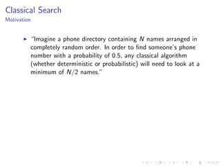
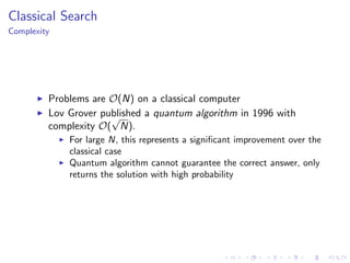
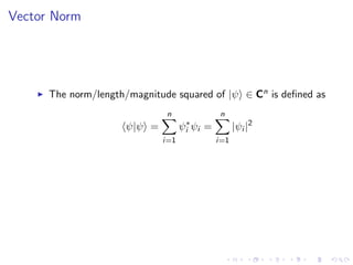
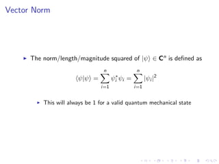
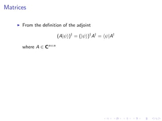
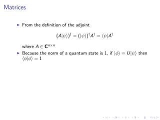
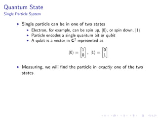
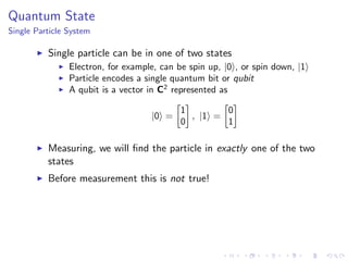
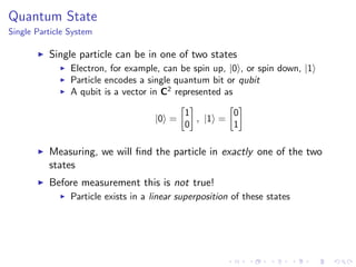
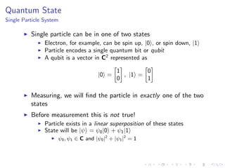
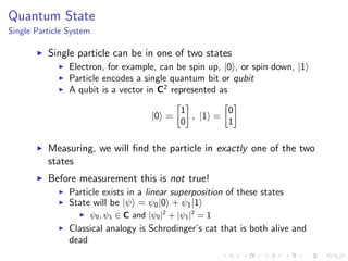
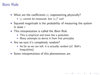
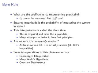
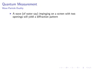
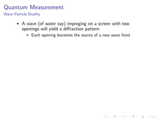
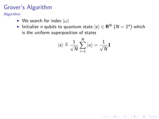
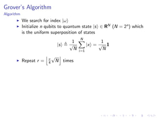
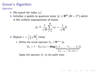
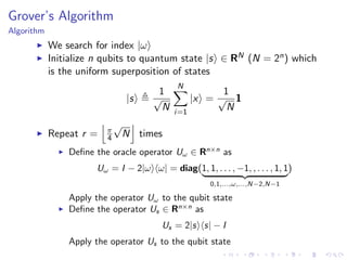
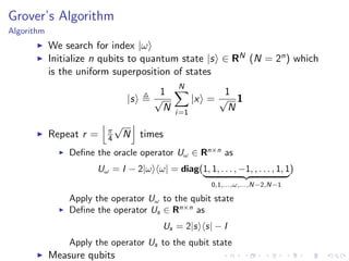
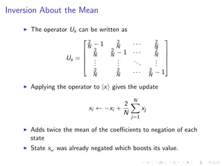
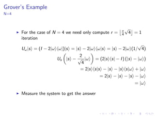
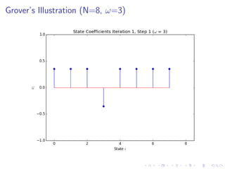
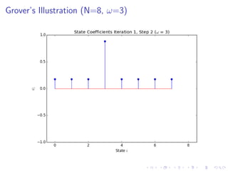
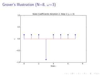
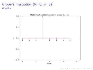
Grover's algorithm - Introduction to quantum computingMeir TOLEDANO
An introduction to quantum computing by the grover's algorithm. I am explaining the expected performance boost on quantum computer. I also review the practical implementation of QBit as of 2020. I also shares some figure about the economics of quantum technologies.
Shor's algorithm is for quantum computer. Using this algorithm any arbitrarily large number can be factored in polynomial time. which is not possible in classical computer
In this deck from the Argonne Training Program on Extreme-Scale Computing 2019, Jonathan Baker from the University of Chicago presents: Quantum Computing: The Why and How.
"Jonathan Baker is a second year Ph.D student at The University of Chicago advised by Fred Chong. He is studying quantum architectures, specifically how to map quantum algorithms more efficiently to near term devices. Additionally, he is interested in multivalued logic and taking advantage of quantum computing’s natural access to higher order states and using these states to make computation more efficient. Prior to beginning his Ph.D., he studied at the University of Notre Dame where he obtained a B.S. of Engineering in computer science and a B.S. in Chemistry and Mathematics."
Watch the video: https://wp.me/p3RLHQ-l1i
Learn more: https://extremecomputingtraining.anl.gov/
Sign up for our insideHPC Newsletter: http://insidehpc.com/newsletter
What is the Expectation Maximization (EM) Algorithm?Kazuki Yoshida
Review of Do and Batzoglou. "What is the expectation maximization algorith?" Nat. Biotechnol. 2008;26:897. Also covers the Data Augmentation and Stan implementation. Resources at https://github.com/kaz-yos/em_da_repo
Apresentação sobre Criptografia baseada em reticulados (lattices), realizada no contexto da disciplina de Post-Quantum Cryptography do PPGCC da UFSC.
Versão odp: http://coenc.td.utfpr.edu.br/~giron/presentations/aula_lattice.odp
Quantum computing has become a noteworthy topic in academia and industry. The multinational companies in the world have been obtaining impressive advances in all areas of quantum technology during the last two decades. These companies try to construct real quantum computers in order to exploit their theoretical preferences over today’s classical computers in practical applications. However, they are challenging to build a full-scale quantum computer because of their increased susceptibility to errors due to decoherence and other quantum noise. Therefore, quantum error correction (QEC) and fault-tolerance protocol will be essential for running quantum algorithms on large-scale quantum computers.
The overall effect of noise is modeled in terms of a set of Pauli operators and the identity acting on the physical qubits (bit flip, phase flip and a combination of bit and phase flips). In addition to Pauli errors, there is another error named leakage errors that occur when a qubit leaves the defined computational subspace. As the location of leakage errors is unknown, these can damage even more the quantum computations. Thus, this talk will briefly provide quantum error models.
In computer science and operations research, a genetic algorithm (GA) is a metaheuristic inspired by the process of natural selection that belongs to the larger class of evolutionary algorithms (EA). Genetic algorithms are commonly used to generate high-quality solutions to optimization and search problems by relying on bio-inspired operators such as mutation, crossover and selection.
Introduction to Quantum Computation. Part - 1Arunabha Saha
Introduction to quantum computation. Here the very basic maths described needed for quantum information theory as well as computation. Postulates of quantum mechanics and the Hisenberg`s Uncertainty principle. Basic operator theories are described here.
Random Matrix Theory and Machine Learning - Part 3Fabian Pedregosa
ICML 2021 tutorial on random matrix theory and machine learning.
Part 3 covers: 1. Motivation: Average-case versus worst-case in high dimensions 2. Algorithm halting times (runtimes) 3. Outlook
Mathematics (from Greek μάθημα máthēma, “knowledge, study, learning”) is the study of topics such as quantity (numbers), structure, space, and change. There is a range of views among mathematicians and philosophers as to the exact scope and definition of mathematics
A Probabilistic Algorithm for Computation of Polynomial Greatest Common with ...mathsjournal
In the earlier work, Knuth present an algorithm to decrease the coefficient growth in the Euclidean algorithm of polynomials called subresultant algorithm. However, the output polynomials may have a small factor which can be removed. Then later, Brown of Bell Telephone Laboratories showed the subresultant in another way by adding a variant called 𝜏 and gave a way to compute the variant. Nevertheless, the way failed to determine every 𝜏 correctly.
In this paper, we will give a probabilistic algorithm to determine the variant 𝜏 correctly in most cases by adding a few steps instead of computing 𝑡(𝑥) when given 𝑓(𝑥) and𝑔(𝑥) ∈ ℤ[𝑥], where 𝑡(𝑥) satisfies that 𝑠(𝑥)𝑓(𝑥) + 𝑡(𝑥)𝑔(𝑥) = 𝑟(𝑥), here 𝑡(𝑥), 𝑠(𝑥) ∈ ℤ[𝑥]
Saudi Arabia stands as a titan in the global energy landscape, renowned for its abundant oil and gas resources. It's the largest exporter of petroleum and holds some of the world's most significant reserves. Let's delve into the top 10 oil and gas projects shaping Saudi Arabia's energy future in 2024.
Immunizing Image Classifiers Against Localized Adversary Attacksgerogepatton
This paper addresses the vulnerability of deep learning models, particularly convolutional neural networks
(CNN)s, to adversarial attacks and presents a proactive training technique designed to counter them. We
introduce a novel volumization algorithm, which transforms 2D images into 3D volumetric representations.
When combined with 3D convolution and deep curriculum learning optimization (CLO), itsignificantly improves
the immunity of models against localized universal attacks by up to 40%. We evaluate our proposed approach
using contemporary CNN architectures and the modified Canadian Institute for Advanced Research (CIFAR-10
and CIFAR-100) and ImageNet Large Scale Visual Recognition Challenge (ILSVRC12) datasets, showcasing
accuracy improvements over previous techniques. The results indicate that the combination of the volumetric
input and curriculum learning holds significant promise for mitigating adversarial attacks without necessitating
adversary training.
Hierarchical Digital Twin of a Naval Power SystemKerry Sado
A hierarchical digital twin of a Naval DC power system has been developed and experimentally verified. Similar to other state-of-the-art digital twins, this technology creates a digital replica of the physical system executed in real-time or faster, which can modify hardware controls. However, its advantage stems from distributing computational efforts by utilizing a hierarchical structure composed of lower-level digital twin blocks and a higher-level system digital twin. Each digital twin block is associated with a physical subsystem of the hardware and communicates with a singular system digital twin, which creates a system-level response. By extracting information from each level of the hierarchy, power system controls of the hardware were reconfigured autonomously. This hierarchical digital twin development offers several advantages over other digital twins, particularly in the field of naval power systems. The hierarchical structure allows for greater computational efficiency and scalability while the ability to autonomously reconfigure hardware controls offers increased flexibility and responsiveness. The hierarchical decomposition and models utilized were well aligned with the physical twin, as indicated by the maximum deviations between the developed digital twin hierarchy and the hardware.
Sachpazis:Terzaghi Bearing Capacity Estimation in simple terms with Calculati...Dr.Costas Sachpazis
Terzaghi's soil bearing capacity theory, developed by Karl Terzaghi, is a fundamental principle in geotechnical engineering used to determine the bearing capacity of shallow foundations. This theory provides a method to calculate the ultimate bearing capacity of soil, which is the maximum load per unit area that the soil can support without undergoing shear failure. The Calculation HTML Code included.
Cosmetic shop management system project report.pdfKamal Acharya
Buying new cosmetic products is difficult. It can even be scary for those who have sensitive skin and are prone to skin trouble. The information needed to alleviate this problem is on the back of each product, but it's thought to interpret those ingredient lists unless you have a background in chemistry.
Instead of buying and hoping for the best, we can use data science to help us predict which products may be good fits for us. It includes various function programs to do the above mentioned tasks.
Data file handling has been effectively used in the program.
The automated cosmetic shop management system should deal with the automation of general workflow and administration process of the shop. The main processes of the system focus on customer's request where the system is able to search the most appropriate products and deliver it to the customers. It should help the employees to quickly identify the list of cosmetic product that have reached the minimum quantity and also keep a track of expired date for each cosmetic product. It should help the employees to find the rack number in which the product is placed.It is also Faster and more efficient way.
3. Classical Search
Motivation
“Imagine a phone directory containing N names arranged in
completely random order. In order to find someone’s phone
number with a probability of 0.5, any classical algorithm
(whether deterministic or probabilistic) will need to look at a
minimum of N/2 names.”
4. Classical Search
Motivation
“Imagine a phone directory containing N names arranged in
completely random order. In order to find someone’s phone
number with a probability of 0.5, any classical algorithm
(whether deterministic or probabilistic) will need to look at a
minimum of N/2 names.”
Consider the function F : {0, 1}3 → {0, 1},
F(x, y, z) =(x ∨ y ∨ z)∧
(¬x ∨ ¬y ∨ z)∧
(x ∨ ¬y ∨ ¬z)∧
(¬x ∨ y ∨ ¬z)
Question: For what values of the input does F(x, y, z) = 1?
5. Classical Search
Complexity
Problems are O(N) on a classical computer
Lov Grover published a quantum algorithm in 1996 with
complexity O(
√
N).
For large N, this represents a significant improvement over the
classical case
Quantum algorithm cannot guarantee the correct answer, only
returns the solution with high probability
9. Notation
R is set of real numbers
C is set of complex numbers (e.g. x + iy)
10. Notation
R is set of real numbers
C is set of complex numbers (e.g. x + iy)
Rn (Cn) indicates column vector of n real (complex) numbers
respectively
11. Notation
R is set of real numbers
C is set of complex numbers (e.g. x + iy)
Rn (Cn) indicates column vector of n real (complex) numbers
respectively
z∗ is the complex conjugate
If z = x + iy then z∗
= x − iy
12. Notation
R is set of real numbers
C is set of complex numbers (e.g. x + iy)
Rn (Cn) indicates column vector of n real (complex) numbers
respectively
z∗ is the complex conjugate
If z = x + iy then z∗
= x − iy
|ψ is Dirac notation for a column vector (ket vector)
13. Notation
R is set of real numbers
C is set of complex numbers (e.g. x + iy)
Rn (Cn) indicates column vector of n real (complex) numbers
respectively
z∗ is the complex conjugate
If z = x + iy then z∗
= x − iy
|ψ is Dirac notation for a column vector (ket vector)
ψ| is Dirac notation for a row vector (bra vector)
14. Notation (cont’d)
A ∈ Rm×n(Cm×n) means A is a matrix of real (complex)
numbers with m rows and n columns
15. Notation (cont’d)
A ∈ Rm×n(Cm×n) means A is a matrix of real (complex)
numbers with m rows and n columns
When m = n we call A an operator
16. Notation (cont’d)
A ∈ Rm×n(Cm×n) means A is a matrix of real (complex)
numbers with m rows and n columns
When m = n we call A an operator
A† is Hermitian/adjoint/conjugate transpose of A
17. Notation (cont’d)
A ∈ Rm×n(Cm×n) means A is a matrix of real (complex)
numbers with m rows and n columns
When m = n we call A an operator
A† is Hermitian/adjoint/conjugate transpose of A
If a matrix A has elements Aij the matrix A†
has entries A∗
ji
An example is ψ| = |ψ †
18. Notation (cont’d)
A ∈ Rm×n(Cm×n) means A is a matrix of real (complex)
numbers with m rows and n columns
When m = n we call A an operator
A† is Hermitian/adjoint/conjugate transpose of A
If a matrix A has elements Aij the matrix A†
has entries A∗
ji
An example is ψ| = |ψ †
The quantity φ|ψ is called the inner product
The quantity is a scalar with value
n
i=1 φ∗
i ψi
21. Vector Norm
The norm/length/magnitude squared of |ψ ∈ Cn is defined as
ψ|ψ =
n
i=1
ψ∗
i ψi =
n
i=1
|ψi |2
This will always be 1 for a valid quantum mechanical state
23. Matrices
From the definition of the adjoint
(A|ψ )†
= (|ψ )†
A†
= ψ|A†
where A ∈ Cn×n
Because the norm of a quantum state is 1, if |φ = U|ψ then
φ|φ = 1
24. Matrices
From the definition of the adjoint
(A|ψ )†
= (|ψ )†
A†
= ψ|A†
where A ∈ Cn×n
Because the norm of a quantum state is 1, if |φ = U|ψ then
φ|φ = 1
From this we have ( ψ|U†
)(U|ψ ) = 1 which means UT
U = I
25. Matrices
From the definition of the adjoint
(A|ψ )†
= (|ψ )†
A†
= ψ|A†
where A ∈ Cn×n
Because the norm of a quantum state is 1, if |φ = U|ψ then
φ|φ = 1
From this we have ( ψ|U†
)(U|ψ ) = 1 which means UT
U = I
An operator satisfying this property is called unitary
26. Matrices
From the definition of the adjoint
(A|ψ )†
= (|ψ )†
A†
= ψ|A†
where A ∈ Cn×n
Because the norm of a quantum state is 1, if |φ = U|ψ then
φ|φ = 1
From this we have ( ψ|U†
)(U|ψ ) = 1 which means UT
U = I
An operator satisfying this property is called unitary
Unitary operators are the way in which quantum states are
altered or evolved
H =
1
√
2
1 1
1 −1
, σx =
0 1
1 0
, σy =
0 i
−i 0
, σz =
1 0
0 −1
28. Linearity
Linearity of a function f means
f (x + y) = f (x) + f (y)
f (αx) = αf (x)
Matrix multiplication is linear
29. Linearity
Linearity of a function f means
f (x + y) = f (x) + f (y)
f (αx) = αf (x)
Matrix multiplication is linear
Common modeling approximation in engineering
Example: log(1 + x) is very nearly x for small x
30. Linearity & QM
Linearity is a fundamental property of QM
“With classical fields, we often use linear equations,
such as the differential equations that allow us to
solve for small oscillatory motion of, say, a pendu-
lum. In such a classical case, the linear equation is
an approximation; a pendulum with twice the am-
plitude of oscillation will not oscillate at exactly the
same frequency, for example. Hence we cannot take
the solution derived at one amplitude of oscillation of
the pendulum and merely scale it up for larger ampli-
tudes of oscillation, except as a first approximation.
We should emphasize right away, however, that, in
quantum mechanics, this linearity of the equations
with respect to the quantum mechanical amplitude
is not an approximation of any kind; it is apparently
an absolute property.”-David Miller (Prof. Stanford
University)
33. Quantum State
Single Particle System
Single particle can be in one of two states
Electron, for example, can be spin up, |0 , or spin down, |1
34. Quantum State
Single Particle System
Single particle can be in one of two states
Electron, for example, can be spin up, |0 , or spin down, |1
Particle encodes a single quantum bit or qubit
35. Quantum State
Single Particle System
Single particle can be in one of two states
Electron, for example, can be spin up, |0 , or spin down, |1
Particle encodes a single quantum bit or qubit
A qubit is a vector in C2
represented as
|0 =
1
0
, |1 =
0
1
36. Quantum State
Single Particle System
Single particle can be in one of two states
Electron, for example, can be spin up, |0 , or spin down, |1
Particle encodes a single quantum bit or qubit
A qubit is a vector in C2
represented as
|0 =
1
0
, |1 =
0
1
Measuring, we will find the particle in exactly one of the two
states
37. Quantum State
Single Particle System
Single particle can be in one of two states
Electron, for example, can be spin up, |0 , or spin down, |1
Particle encodes a single quantum bit or qubit
A qubit is a vector in C2
represented as
|0 =
1
0
, |1 =
0
1
Measuring, we will find the particle in exactly one of the two
states
Before measurement this is not true!
38. Quantum State
Single Particle System
Single particle can be in one of two states
Electron, for example, can be spin up, |0 , or spin down, |1
Particle encodes a single quantum bit or qubit
A qubit is a vector in C2
represented as
|0 =
1
0
, |1 =
0
1
Measuring, we will find the particle in exactly one of the two
states
Before measurement this is not true!
Particle exists in a linear superposition of these states
39. Quantum State
Single Particle System
Single particle can be in one of two states
Electron, for example, can be spin up, |0 , or spin down, |1
Particle encodes a single quantum bit or qubit
A qubit is a vector in C2
represented as
|0 =
1
0
, |1 =
0
1
Measuring, we will find the particle in exactly one of the two
states
Before measurement this is not true!
Particle exists in a linear superposition of these states
State will be |ψ = ψ0|0 + ψ1|1
ψ0, ψ1 ∈ C and |ψ0|2
+ |ψ1|2
= 1
40. Quantum State
Single Particle System
Single particle can be in one of two states
Electron, for example, can be spin up, |0 , or spin down, |1
Particle encodes a single quantum bit or qubit
A qubit is a vector in C2
represented as
|0 =
1
0
, |1 =
0
1
Measuring, we will find the particle in exactly one of the two
states
Before measurement this is not true!
Particle exists in a linear superposition of these states
State will be |ψ = ψ0|0 + ψ1|1
ψ0, ψ1 ∈ C and |ψ0|2
+ |ψ1|2
= 1
Classical analogy is Schrodinger’s cat that is both alive and
dead
43. Quantum State
Multi-Particle System
Suppose we have n particles each of which can be in one of
two states
The system represents n qubits of information
There are N = 2n
possible different states
|0 . . . 00 , |0 . . . 01 , |0 . . . 10 , . . . , |1 . . . 11
44. Quantum State
Multi-Particle System
Suppose we have n particles each of which can be in one of
two states
The system represents n qubits of information
There are N = 2n
possible different states
|0 . . . 00 , |0 . . . 01 , |0 . . . 10 , . . . , |1 . . . 11
Each state is a standard basis vector in RN
(i.e. one
component equal to 1 and the rest 0)
Note: The vector components are not the same as the entries
of the Dirac notation
45. Quantum State
Multi-Particle System
Suppose we have n particles each of which can be in one of
two states
The system represents n qubits of information
There are N = 2n
possible different states
|0 . . . 00 , |0 . . . 01 , |0 . . . 10 , . . . , |1 . . . 11
Each state is a standard basis vector in RN
(i.e. one
component equal to 1 and the rest 0)
Note: The vector components are not the same as the entries
of the Dirac notation
Measuring, we will find the system to be in one of N = 2n
possible states |ψ ∈ RN
46. Quantum State
Multi-Particle System
Suppose we have n particles each of which can be in one of
two states
The system represents n qubits of information
There are N = 2n
possible different states
|0 . . . 00 , |0 . . . 01 , |0 . . . 10 , . . . , |1 . . . 11
Each state is a standard basis vector in RN
(i.e. one
component equal to 1 and the rest 0)
Note: The vector components are not the same as the entries
of the Dirac notation
Measuring, we will find the system to be in one of N = 2n
possible states |ψ ∈ RN
Before measurement, it will be in a linear superposition of
these states
47. Quantum State
Multi-Particle System
Suppose we have n particles each of which can be in one of
two states
The system represents n qubits of information
There are N = 2n
possible different states
|0 . . . 00 , |0 . . . 01 , |0 . . . 10 , . . . , |1 . . . 11
Each state is a standard basis vector in RN
(i.e. one
component equal to 1 and the rest 0)
Note: The vector components are not the same as the entries
of the Dirac notation
Measuring, we will find the system to be in one of N = 2n
possible states |ψ ∈ RN
Before measurement, it will be in a linear superposition of
these states
Its state will be
|ψ = ψ0|0 . . . 00 + ψ1|0 . . . 01 + · · · + ψN−1|1 . . . 11 where
ψi ∈ C and
N−1
i=0 |ψi |2
= 1
49. Born Rule
What are the coefficients ψi respresenting physically?
ψi cannot be measured, but |ψi |2
can!
50. Born Rule
What are the coefficients ψi respresenting physically?
ψi cannot be measured, but |ψi |2
can!
Squared magnitude is the probability of measuring the system
in state i
51. Born Rule
What are the coefficients ψi respresenting physically?
ψi cannot be measured, but |ψi |2
can!
Squared magnitude is the probability of measuring the system
in state i
This interpretation is called the Born Rule
52. Born Rule
What are the coefficients ψi respresenting physically?
ψi cannot be measured, but |ψi |2
can!
Squared magnitude is the probability of measuring the system
in state i
This interpretation is called the Born Rule
This is empirical and more like a postulate
53. Born Rule
What are the coefficients ψi respresenting physically?
ψi cannot be measured, but |ψi |2
can!
Squared magnitude is the probability of measuring the system
in state i
This interpretation is called the Born Rule
This is empirical and more like a postulate
Many attempts to derive it from first principles
54. Born Rule
What are the coefficients ψi respresenting physically?
ψi cannot be measured, but |ψi |2
can!
Squared magnitude is the probability of measuring the system
in state i
This interpretation is called the Born Rule
This is empirical and more like a postulate
Many attempts to derive it from first principles
Are we sure it’s completely random?
55. Born Rule
What are the coefficients ψi respresenting physically?
ψi cannot be measured, but |ψi |2
can!
Squared magnitude is the probability of measuring the system
in state i
This interpretation is called the Born Rule
This is empirical and more like a postulate
Many attempts to derive it from first principles
Are we sure it’s completely random?
As far as we can tell, it is actually random (cf. Bell’s
Inequalities)
56. Born Rule
What are the coefficients ψi respresenting physically?
ψi cannot be measured, but |ψi |2
can!
Squared magnitude is the probability of measuring the system
in state i
This interpretation is called the Born Rule
This is empirical and more like a postulate
Many attempts to derive it from first principles
Are we sure it’s completely random?
As far as we can tell, it is actually random (cf. Bell’s
Inequalities)
Some interpretations of this phenomenon are
57. Born Rule
What are the coefficients ψi respresenting physically?
ψi cannot be measured, but |ψi |2
can!
Squared magnitude is the probability of measuring the system
in state i
This interpretation is called the Born Rule
This is empirical and more like a postulate
Many attempts to derive it from first principles
Are we sure it’s completely random?
As far as we can tell, it is actually random (cf. Bell’s
Inequalities)
Some interpretations of this phenomenon are
Copenhagen Interpretation
Many World’s Hypothesis
Quantum Decoherence
58. Quantum Measurement
Wave Particle Duality
A wave (of water say) impinging on a screen with two
openings will yield a diffraction pattern
59. Quantum Measurement
Wave Particle Duality
A wave (of water say) impinging on a screen with two
openings will yield a diffraction pattern
Each opening becomes the source of a new wave front
60. Quantum Measurement
Wave Particle Duality
A wave (of water say) impinging on a screen with two
openings will yield a diffraction pattern
Each opening becomes the source of a new wave front
The two waves interfere with each other forming alternating
peaks and troughs
61. Quantum Measurement
Wave Particle Duality
A wave (of water say) impinging on a screen with two
openings will yield a diffraction pattern
Each opening becomes the source of a new wave front
The two waves interfere with each other forming alternating
peaks and troughs
63. Quantum Measurement (cont’d)
Wave Particle Duality
Perform the same experiment with an electron gun
A diffraction pattern is observed!
This indicates electrons are like waves
64. Quantum Measurement (cont’d)
Wave Particle Duality
Perform the same experiment with an electron gun
A diffraction pattern is observed!
This indicates electrons are like waves
Now we have an apparatus that can shoot only a single
electron at a time
65. Quantum Measurement (cont’d)
Wave Particle Duality
Perform the same experiment with an electron gun
A diffraction pattern is observed!
This indicates electrons are like waves
Now we have an apparatus that can shoot only a single
electron at a time
A diffraction pattern! The electron is interfering with itself
66. Quantum Measurement (cont’d)
Wave Particle Duality
Perform the same experiment with an electron gun
A diffraction pattern is observed!
This indicates electrons are like waves
Now we have an apparatus that can shoot only a single
electron at a time
A diffraction pattern! The electron is interfering with itself
A measurement device is placed on one of the slits to see
which one the electron went through
67. Quantum Measurement (cont’d)
Wave Particle Duality
Perform the same experiment with an electron gun
A diffraction pattern is observed!
This indicates electrons are like waves
Now we have an apparatus that can shoot only a single
electron at a time
A diffraction pattern! The electron is interfering with itself
A measurement device is placed on one of the slits to see
which one the electron went through
Diffraction pattern is gone.
Electron behaves like a particle that goes through one slit or
the other when measured
The act of measurement has altered the outcome
72. Grover’s Algorithm
Function Inversion
Often framed in the context of unstructured database search
More precisely, searches a function for a single satisfying input
Given y, find the corresponding x such that f (x) = y.
Invert the function f (·)
To search an explicit list (i.e. unstructured database), need a
function backing it
73. Grover’s Algorithm
Function Inversion
Often framed in the context of unstructured database search
More precisely, searches a function for a single satisfying input
Given y, find the corresponding x such that f (x) = y.
Invert the function f (·)
To search an explicit list (i.e. unstructured database), need a
function backing it
If there is no solution or multiple solutions, algorithm does not
work out of the box
76. Grover’s Algorithm
Algorithm
We search for index |ω
Initialize n qubits to quantum state |s ∈ RN (N = 2n) which
is the uniform superposition of states
|s
1
√
N
N
i=1
|x =
1
√
N
1
77. Grover’s Algorithm
Algorithm
We search for index |ω
Initialize n qubits to quantum state |s ∈ RN (N = 2n) which
is the uniform superposition of states
|s
1
√
N
N
i=1
|x =
1
√
N
1
Repeat r = π
4
√
N times
78. Grover’s Algorithm
Algorithm
We search for index |ω
Initialize n qubits to quantum state |s ∈ RN (N = 2n) which
is the uniform superposition of states
|s
1
√
N
N
i=1
|x =
1
√
N
1
Repeat r = π
4
√
N times
Define the oracle operator Uω ∈ Rn×n
as
Uω = I − 2|ω ω| = diag(1, 1, . . . , −1, , . . . , 1, 1
0,1,...,ω,...,N−2,N−1
)
Apply the operator Uω to the qubit state
79. Grover’s Algorithm
Algorithm
We search for index |ω
Initialize n qubits to quantum state |s ∈ RN (N = 2n) which
is the uniform superposition of states
|s
1
√
N
N
i=1
|x =
1
√
N
1
Repeat r = π
4
√
N times
Define the oracle operator Uω ∈ Rn×n
as
Uω = I − 2|ω ω| = diag(1, 1, . . . , −1, , . . . , 1, 1
0,1,...,ω,...,N−2,N−1
)
Apply the operator Uω to the qubit state
Define the operator Us ∈ Rn×n
as
Us = 2|s s| − I
Apply the operator Us to the qubit state
80. Grover’s Algorithm
Algorithm
We search for index |ω
Initialize n qubits to quantum state |s ∈ RN (N = 2n) which
is the uniform superposition of states
|s
1
√
N
N
i=1
|x =
1
√
N
1
Repeat r = π
4
√
N times
Define the oracle operator Uω ∈ Rn×n
as
Uω = I − 2|ω ω| = diag(1, 1, . . . , −1, , . . . , 1, 1
0,1,...,ω,...,N−2,N−1
)
Apply the operator Uω to the qubit state
Define the operator Us ∈ Rn×n
as
Us = 2|s s| − I
Apply the operator Us to the qubit state
Measure qubits
81. Inversion About the Mean
The operator Us can be written as
Us =
2
N − 1 2
N · · · 2
N
2
N
2
N − 1 · · · 2
N
...
...
...
...
2
N
2
N · · · 2
N − 1
Applying the operator to |x gives the update
xi ← −xi +
2
N
N
j=1
xj
Adds twice the mean of the coefficients to negation of each
state
State xω was already negated which boosts its value.
82. Grover’s Example
N=4
For the case of N = 4 we need only compute r = π
4
√
4 = 1
iteration
Uω|s = (I − 2|ω ω|)|s = |s − 2|ω ω|s = |s − 2|ω (1/
√
4)
Us |s −
2
√
4
|ω = (2|s s| − I) (|s − |ω )
= 2|s s|s − |s − |s s|ω + |ω
= 2|s − |s − |s − |ω
= |ω
Measure the system to get the answer
89. Grover’s Algorithm
Notes
If the solution does not exist, an answer is returned at random
Performing more iterations will degrade the solution
probability
90. Grover’s Algorithm
Notes
If the solution does not exist, an answer is returned at random
Performing more iterations will degrade the solution
probability
Multiple solutions will change the optimal number of
iterations needed
91. The Quantum Oracle
The oracle is a (problem dependent) function such that
f (ω) = 1 and 0 otherwise
92. The Quantum Oracle
The oracle is a (problem dependent) function such that
f (ω) = 1 and 0 otherwise
Each state is then multiplied with (−1)f (x)
to “mark” the
solution
93. The Quantum Oracle
The oracle is a (problem dependent) function such that
f (ω) = 1 and 0 otherwise
Each state is then multiplied with (−1)f (x)
to “mark” the
solution
Quantum oracle must be able to evaluate on the superposition
of indices
94. The Quantum Oracle
The oracle is a (problem dependent) function such that
f (ω) = 1 and 0 otherwise
Each state is then multiplied with (−1)f (x)
to “mark” the
solution
Quantum oracle must be able to evaluate on the superposition
of indices
Classically, we can only evaluate one query at a time
95. The Quantum Oracle
The oracle is a (problem dependent) function such that
f (ω) = 1 and 0 otherwise
Each state is then multiplied with (−1)f (x)
to “mark” the
solution
Quantum oracle must be able to evaluate on the superposition
of indices
Classically, we can only evaluate one query at a time
QM has natural parallelism; if f can evaluate x or y, then we
can evaluate f 1√
2
(x + y)
96. The Quantum Oracle
The oracle is a (problem dependent) function such that
f (ω) = 1 and 0 otherwise
Each state is then multiplied with (−1)f (x)
to “mark” the
solution
Quantum oracle must be able to evaluate on the superposition
of indices
Classically, we can only evaluate one query at a time
QM has natural parallelism; if f can evaluate x or y, then we
can evaluate f 1√
2
(x + y)
A quantum circuit with quantum gates can be built to
evaluate the predicate
97. The Quantum Oracle
The oracle is a (problem dependent) function such that
f (ω) = 1 and 0 otherwise
Each state is then multiplied with (−1)f (x)
to “mark” the
solution
Quantum oracle must be able to evaluate on the superposition
of indices
Classically, we can only evaluate one query at a time
QM has natural parallelism; if f can evaluate x or y, then we
can evaluate f 1√
2
(x + y)
A quantum circuit with quantum gates can be built to
evaluate the predicate
Gates such as Hadamard, Pauli Spin, Phase shift, CNOT etc
(all are unitary operators) used to build oracles
98. The Quantum Oracle
The oracle is a (problem dependent) function such that
f (ω) = 1 and 0 otherwise
Each state is then multiplied with (−1)f (x)
to “mark” the
solution
Quantum oracle must be able to evaluate on the superposition
of indices
Classically, we can only evaluate one query at a time
QM has natural parallelism; if f can evaluate x or y, then we
can evaluate f 1√
2
(x + y)
A quantum circuit with quantum gates can be built to
evaluate the predicate
Gates such as Hadamard, Pauli Spin, Phase shift, CNOT etc
(all are unitary operators) used to build oracles
Programming a quantum computer is more like programming
an FPGA than writing software
99. Usefulness of Grover’s
The O(
√
N) bound assumes predicate can be evaluated on
superposition of all states
100. Usefulness of Grover’s
The O(
√
N) bound assumes predicate can be evaluated on
superposition of all states
f (·) must be implemented in quantum hardware using
quantum gates
May be difficult to find compact gate representation
Problems like database search must first convert to an implicit
list
Cost of evaluating f (·) may dominate
101. Current State of Quantum Computing
IBM claims to have a working prototype of a 50 qubit
quantum computer
102. Current State of Quantum Computing
IBM claims to have a working prototype of a 50 qubit
quantum computer
D Wave solves optimization problems by exploiting QM effects
103. Current State of Quantum Computing
IBM claims to have a working prototype of a 50 qubit
quantum computer
D Wave solves optimization problems by exploiting QM effects
Much of quantum computing is still theoretical and uses
simulation
Q#, Libquantum, IBM Q etc
Simulation requires lots of memory (e.g. 32 qubits implies
2 · 232
real numbers)