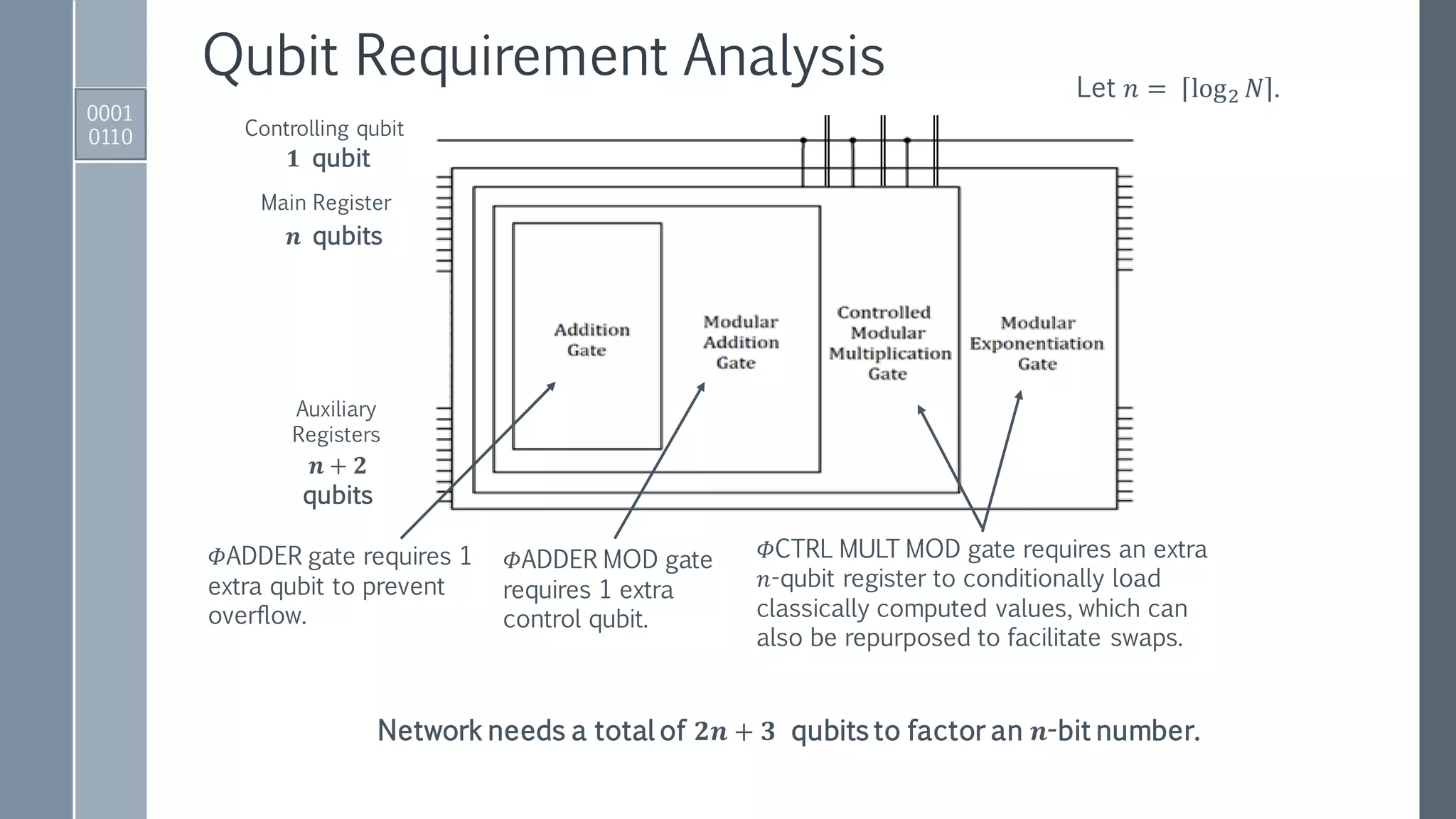
This document provides an exposition on Shor's algorithm and its implementation using quantum circuits and various quantum programming tools including Rigetti's Pyquil, Microsoft's Q#/C#, and IBM's Qiskit. It covers quantum arithmetic circuits, detailed descriptions of Shor's algorithm, and classical examples for understanding the quantum period finding process. Additionally, it discusses the architecture and qubit requirements for successfully factoring large numbers using quantum computing techniques.

1. Shor’s Algorithm
Exposition on Quantum Circuits in
Daniel Hutama
daniel.hutama@mail.mcgill.ca
August 22, 2018
0000
0001

2. Content
› 1. Some Quantum Programming Tools (5 min)
– Rigetti pyQuil
– Microsoft Q#/C#
– IBM QISKit
› 2. Introduction/Shor’s Algorithm Recap (10 min)
– High level overview
› 3. Quantum Arithmetic Circuits (45 min)
– Classical-based reversible designs
– Fourier space improvements
› 4. Appendix
– Shor’s Algorithm detailed description
– Shor’s Algorithm full-stack example
– RSA Cryptosystem – application of the factoring problem
0000
0010

3. 1. Some Quantum Programming Tools
0000
0011
Full list and in-depth descriptions:
https://github.com/markf94/os_quantum_software

4. Python – pyQuil (Rigetti Forest Toolkit)
0000
0100
• Open source Python library developed by Rigetti Computing.
• pyQuil code produces programs in Quantum Instruction Language (Quil),
designed to execute on a machine with shared classical/quantum architecture.
• Quil programs can be executed on a cloud-based Quantum Virtual Machine
(classical simulation of a quantum processor, up to 26 qubits).
• Quil programs can also be run on real quantum processing units (8 qubits).
pyQuil architecture schematic:
arXiv: 1608.03355

5. Python – pyQuil (Rigetti Forest Toolkit)
0000
0101
• Open source Python library developed by Rigetti Computing.
• pyQuil code produces programs in Quantum Instruction Language (Quil),
designed to execute on a machine with shared classical/quantum architecture.
• Quil programs can be executed on a cloud-based Quantum Virtual Machine
(classical simulation of a quantum processor, up to 26 qubits).
• Quil programs can also be run on real quantum processing units (8 qubits).
Import pyQuil library functions
Use QVM (classical simulation)
pyQuil Bell state code
Apply Hadamard and CNOT
Print circuit description
Run program on QVM
Print measurement results
Apply measurements

6. Q# and C# (Microsoft)
0000
0110
Quantum code written in Q# for
creating a Bell state
Creates variables that will be
dynamically updated to store the
value of measurement results.
Initializes qubits to desired input states.
Hadamard and CNOT gates for Bell state circuit.
Measurement counts number of agreements
( i.e. count measurements of |00⟩ or |11⟩ ).
Count number of observations of 1 in register 2.
Reset registers to zero state.
Return number of 0 , 1 , and agreements.

7. 0000
0111 Driving the Q# code with C#
Quantum code written in Q# for
creating a Bell state
Need to write a C# code block
that will drive the Q# experiment
and print the results to console
Command line output:
Q# and C# (Microsoft)

8. 0000
1000
Python – QISKit (IBM)
• IBM’s python library with cloud-based functionality for classical simulations
and computations with real quantum processors (IBM Q Experience).
Initializes a 2-qubit quantum register.
Initializes a 2-bit classical register.
Composes circuit with the two registers.
Apply Hadamard and CNOT gates.
Record measurement results in the classical register.
Use locally installed quantum simulator with 10,000 trials.

9. 1. Introduction
Recap of Shor’s Algorithm
0000
1001
Peter Shor

10. Obtaining Factors of 𝑁 via Order Finding
Step 1
Step 3
Step 2
Step 4
Pick some random seed 𝑥:
1 < 𝑥 < 𝑁 with gcd(𝑥, 𝑁) = 1.
Compute 𝑟, the period of 𝑥 (mod 𝑁).
i.e. find 𝑟 s.t. 𝑥 𝑟 ≡ 1 mod 𝑁 .
Check that 𝑟 ≡ 0 mod 2 .
Check that 𝑥 Τ𝑟
2 ≢ ±1 (mod 𝑁) .
𝑝 = gcd 𝑥 Τ𝑟
2 − 1, 𝑁 .
𝑞 = gcd 𝑥 Τ𝑟
2 + 1, 𝑁 .
0000
1010

11. Classical Example: 𝑵 = 𝟏𝟓.
Multiplicative Group Modulo 15
𝟏 < 𝒙 < 𝑵 | 𝒈𝒄𝒅(𝒙, 𝑵) = 𝟏
Random 𝑥 2 3 4 5 6 7 8 9 10 11 12 13 14
gcd(𝑥, 𝟏𝟓) 1 3 1 5 3 1 1 3 5 1 3 1 1
Continue? Y N Y N N Y Y N N Y N Y Y
𝒙 𝟎
𝐦𝐨𝐝 𝟏𝟓 1 1 1 1 1 1 1
𝒙 𝟏 𝐦𝐨𝐝 𝟏𝟓 2 4 7 8 11 13 14
𝒙 𝟐
𝐦𝐨𝐝 𝟏𝟓 4 1 4 4 1 4 1
𝒙 𝟑 𝐦𝐨𝐝 𝟏𝟓 8 4 13 2 11 7 14
𝒙 𝟒
𝐦𝐨𝐝 𝟏𝟓 1 1 1 1 1 1 1
Period 4 2 4 4 2 4 2
𝑝 = gcd(7 ൗ4
2 − 1, 15)
e.g. if 𝑥 = 7:
𝑞 = gcd(7 ൗ4
2 + 1, 15)
0000
1011
Randomly choose 𝒙, such that:

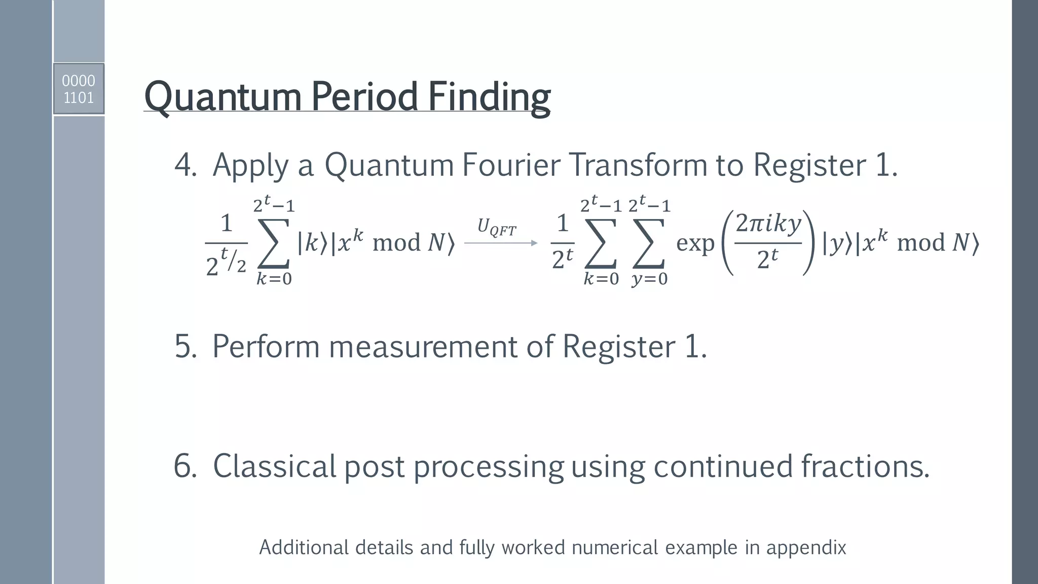
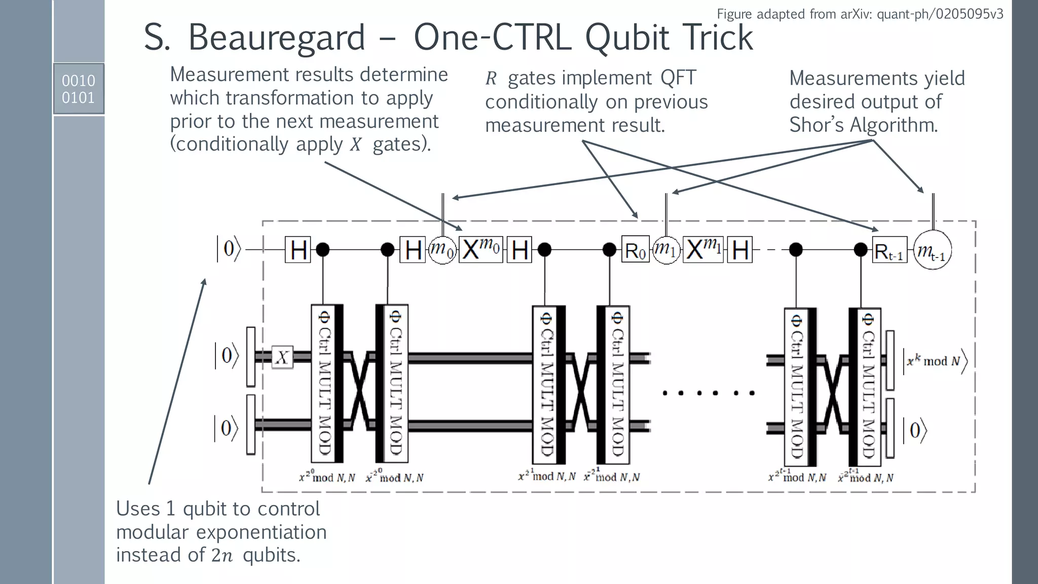
12. Quantum Period Finding
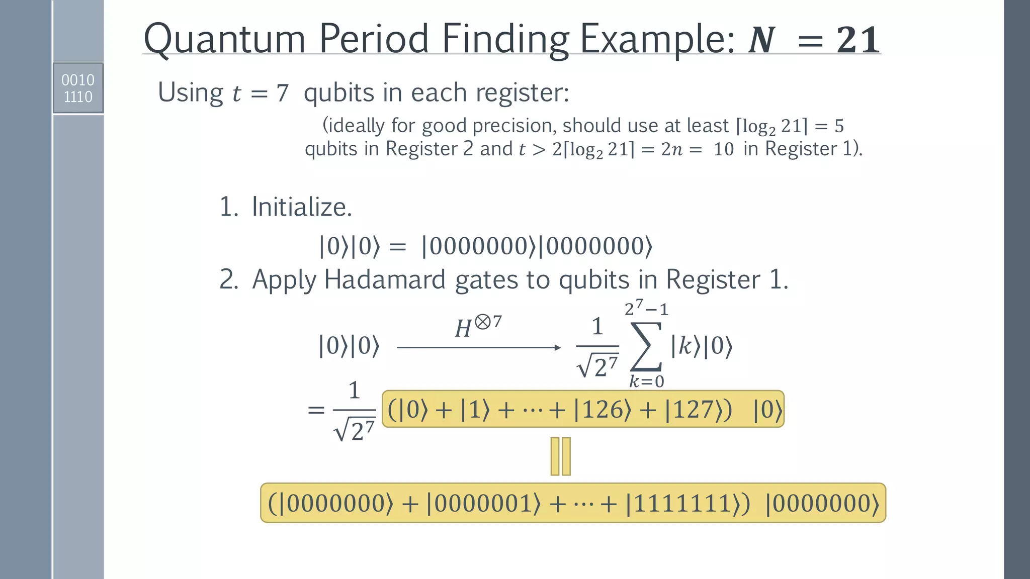
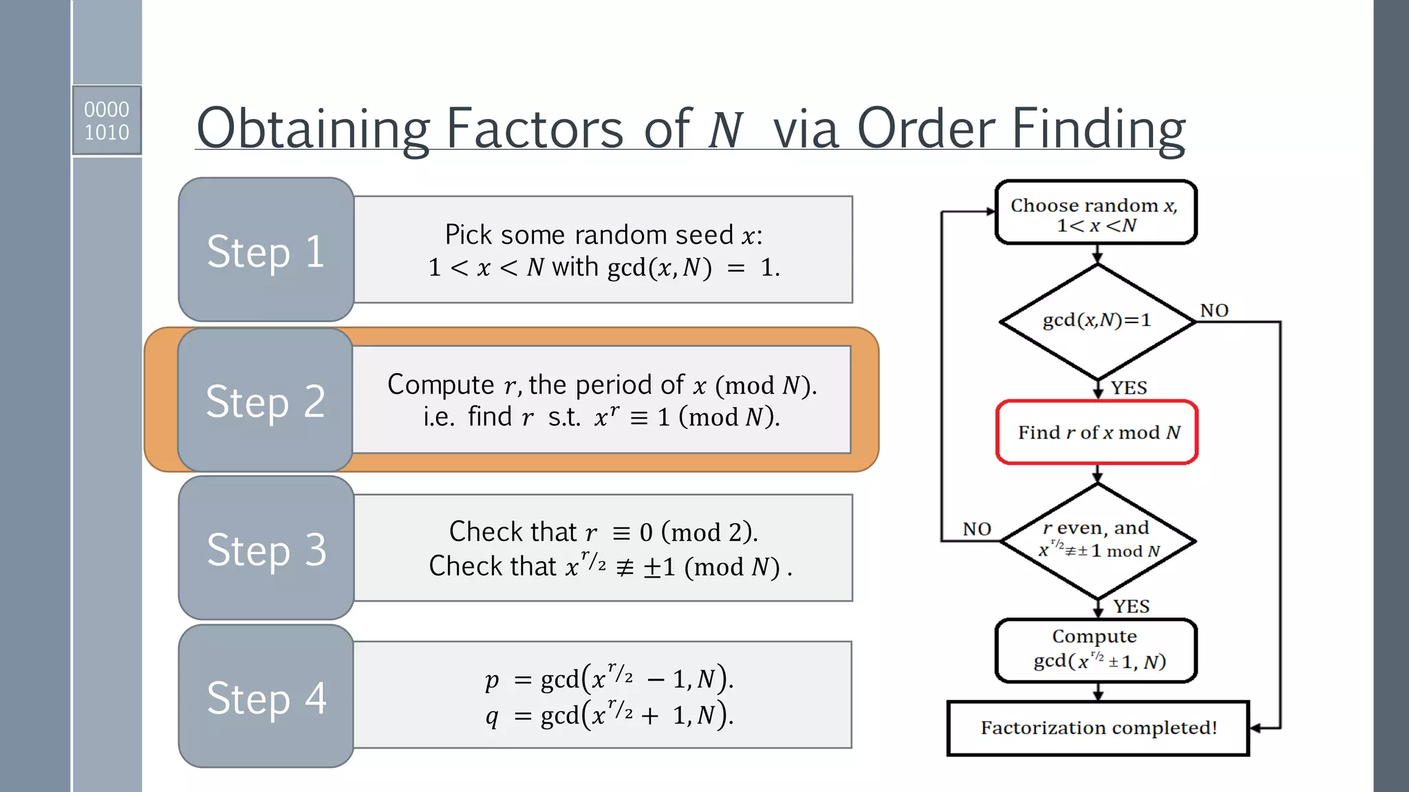
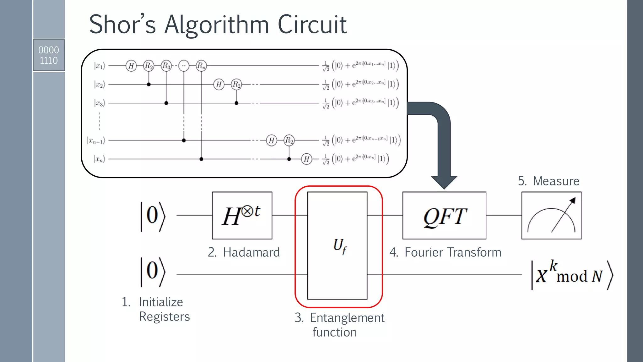
1. Initialize registers to zero-position.
00 … 00 00 …00 = 0 |0⟩
|Register 1⟩ |Register 2⟩
2. Apply Hadamard gates to the 𝑡 qubits in Register 1.
𝑡 qubits in Register 1 to encode
integers [0, …, 2 𝑡
− 1] in binary;
𝑡 larger than 2𝑛 = 2 log2 𝑁 .
0 0
1
2 ൗ𝑡
2
෍
𝑘=0
2 𝑡−1
𝑘 |0⟩
𝐻⊗𝑡
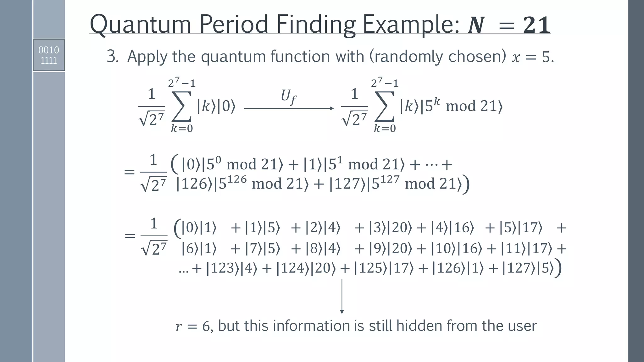
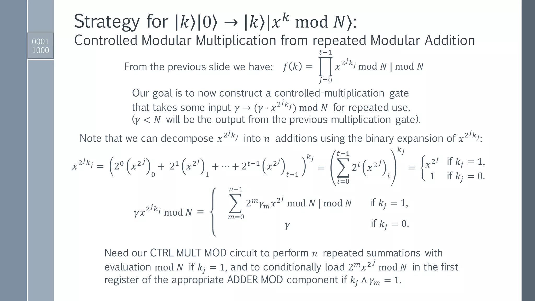
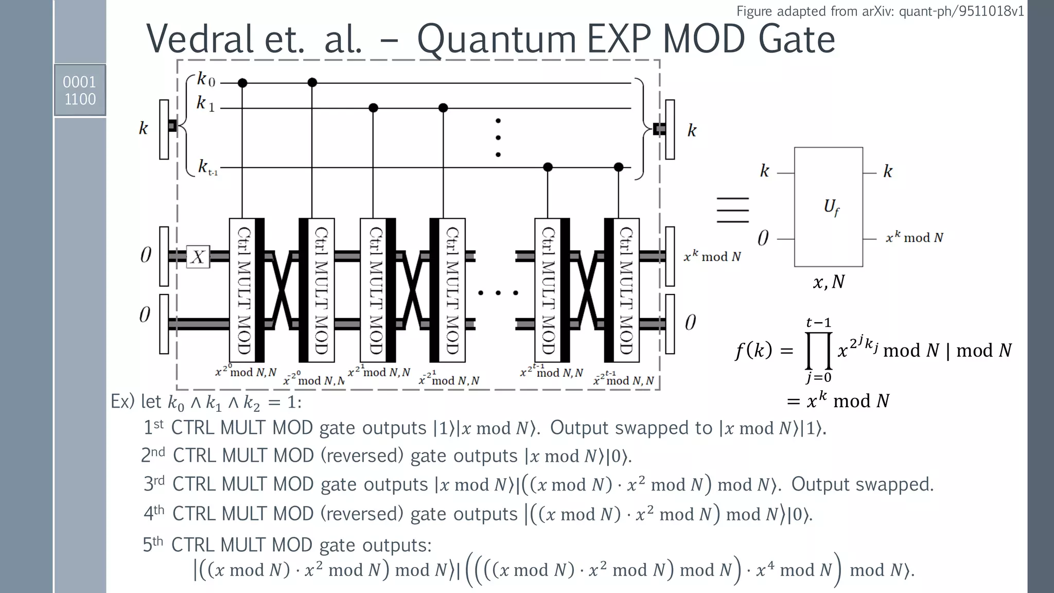
3. Apply a quantum function that performs the map:
𝑈𝑓1
2 ൗ𝑡
2
෍
𝑘=0
2 𝑡−1
𝑘 0
1
2 ൗ𝑡
2
෍
𝑘=0
2 𝑡−1
𝑘 |𝑥 𝑘
mod 𝑁⟩
0000
1100

13. Quantum Period Finding
4. Apply a Quantum Fourier Transform to Register 1.
1
2 ൗ𝑡
2
෍
𝑘=0
2 𝑡−1
𝑘 |𝑥 𝑘
mod 𝑁⟩
1
2 𝑡 ෍
𝑘=0
2 𝑡−1
෍
𝑦=0
2 𝑡−1
exp
2𝜋𝑖𝑘𝑦
2 𝑡
𝑦 |𝑥 𝑘
mod 𝑁⟩
𝑈 𝑄𝐹𝑇
0000
1101
5. Perform measurement of Register 1.
6. Classical post processing using continued fractions.
Additional details and fully worked numerical example in appendix

14. Shor’s Algorithm Circuit
0000
1110
1. Initialize
Registers
2. Hadamard
3. Entanglement
function
4. Fourier Transform
5. Measure

15. 2. Quantum circuits for implementing
𝑘 0 → 𝑘 |x 𝑘
mod 𝑁⟩
0000
1111

16. Gate Set
0001
0000
Pauli X Gate Controlled-NOT Gate Toffoli Gate
Subscripts on a symbol are used to
denote the index of a binary element.
E.g. 𝑘𝑗 ∈ 0,1 is the 𝑗th bit (indexed
from 0) in the binary representation of
the decimal integer 𝑘.
Notation:

17. Level Schematic
0001
0001
Register 1
Register 2
Auxiliary
Registers
|𝑘⟩ |𝑘⟩
|0⟩
|0⟩ |0⟩
|𝑥 𝑘
mod 𝑁⟩
Modules independent
of Register 1 state

18. Vedral et. al. – Quantum ADDER Gate
0001
0010
CARRY gates compute the most
significant bit of 𝑎 + 𝑏 and the
last CARRY stores its value in 𝑏 𝑛
𝑐𝑖
𝑎𝑖
𝑏𝑖
𝑐𝑖+1
𝑐𝑖
𝑎𝑖
𝑏𝑖 ⊕ ai
𝑐𝑖+1 ⊕ (𝑎𝑖∧ 𝑏𝑖) ⊕ (𝑎𝑖 ∧ 𝑐𝑖) ⊕ (𝑏𝑖 ∧ 𝑐𝑖)
𝑐𝑖
𝑎𝑖
𝑏𝑖
𝑐𝑖
𝑎𝑖
𝑏𝑖 ⊕ ai ⊕ 𝑐𝑖
CARRYs reversed to reset
temporary register to 0.
Results of addition stored
in second register.
Figure adapted from arXiv: quant-ph/9511018v1

19. Quantum ADDER Gate
0001
0011
IBM QISKit implementation
CARRY gates to
compute MSB
of 𝑎 + 𝑏
Final CARRY gate
writes the MSB of
𝑎 + 𝑏 to 𝑏3
CNOT to reverse the action
of the final CARRY on 𝑏2
Reversed CARRY gates to reset
temporary register to zero
SUM gates store result
in second register

20. 0001
0100
Vedral et. al. – Quantum ADDER MOD Gate
First ADDER
computes 𝑎 + 𝑏
Second ADDER run in
reverse to subtract 𝑁
MSB used as control for adding back 𝑁
(in the case where 𝑎 + 𝑏 < 𝑁), or adding
zero (in the case where 𝑎 + 𝑏 > 𝑁).
Final components reset
auxiliary qubit to zero
Figure adapted from arXiv: quant-ph/9511018v1

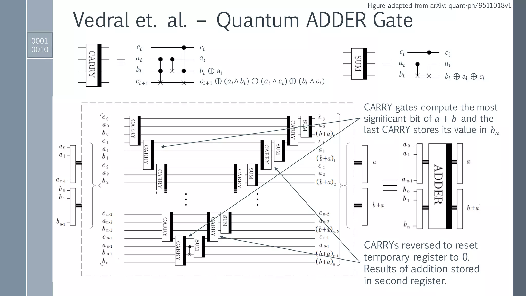
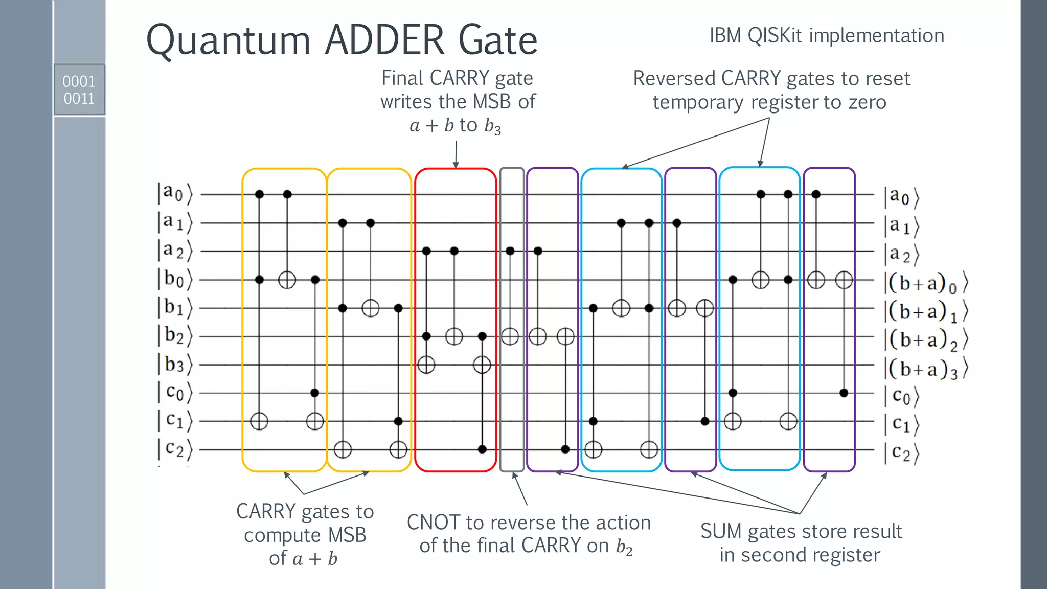
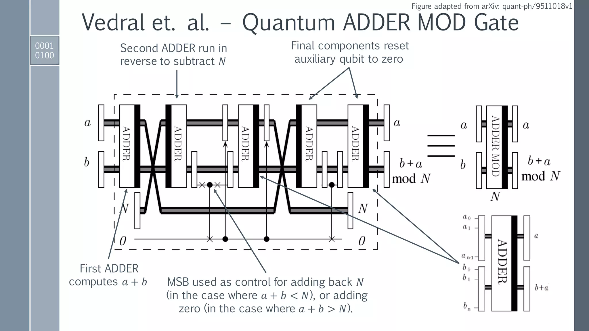
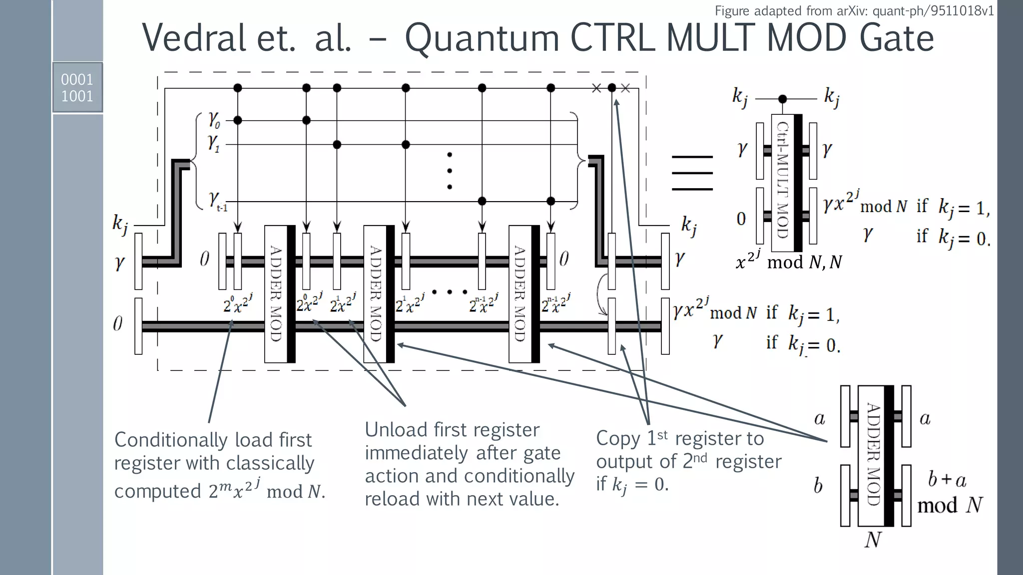
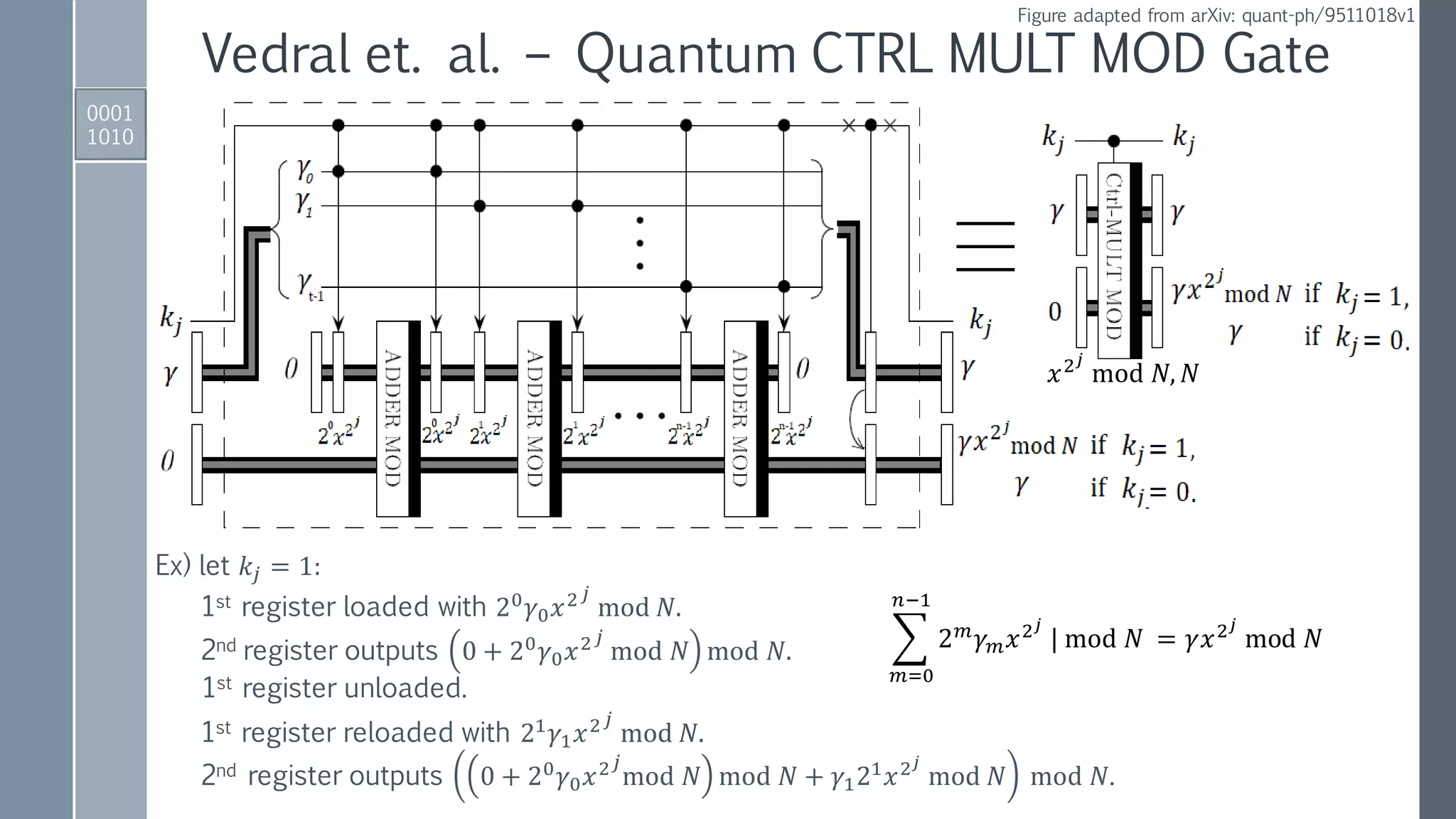
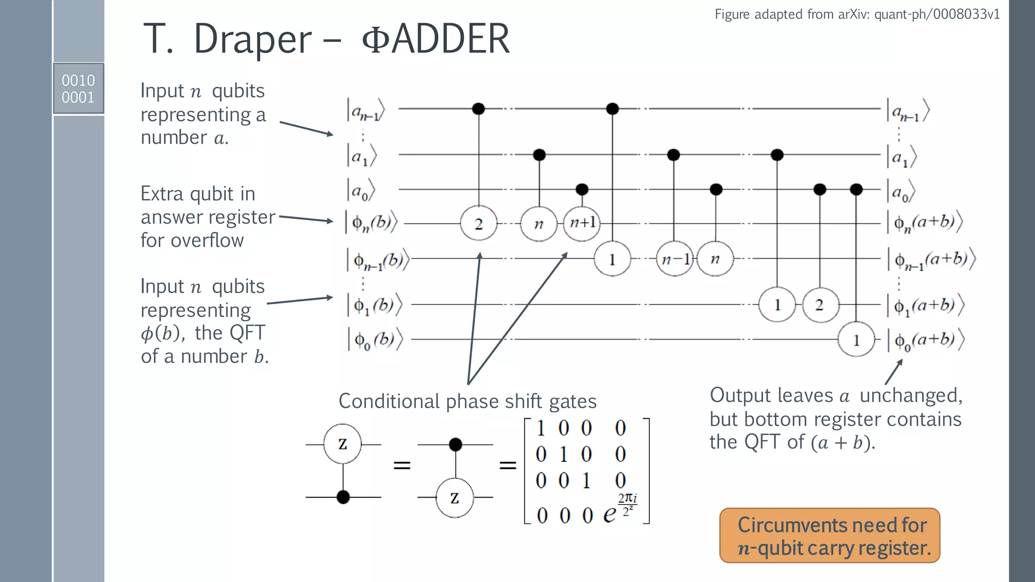
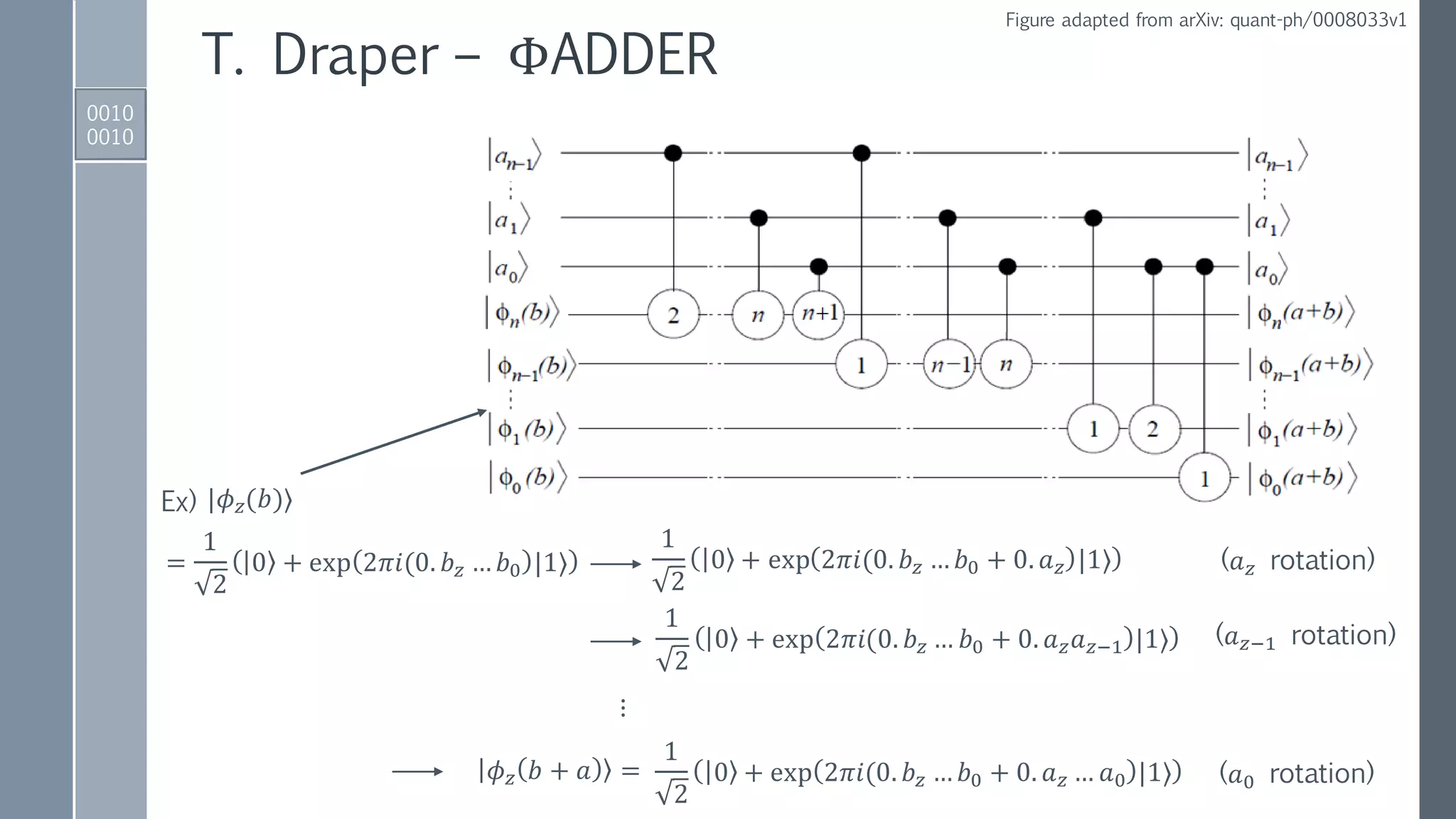
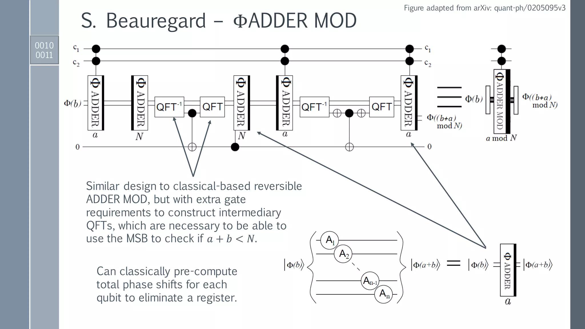
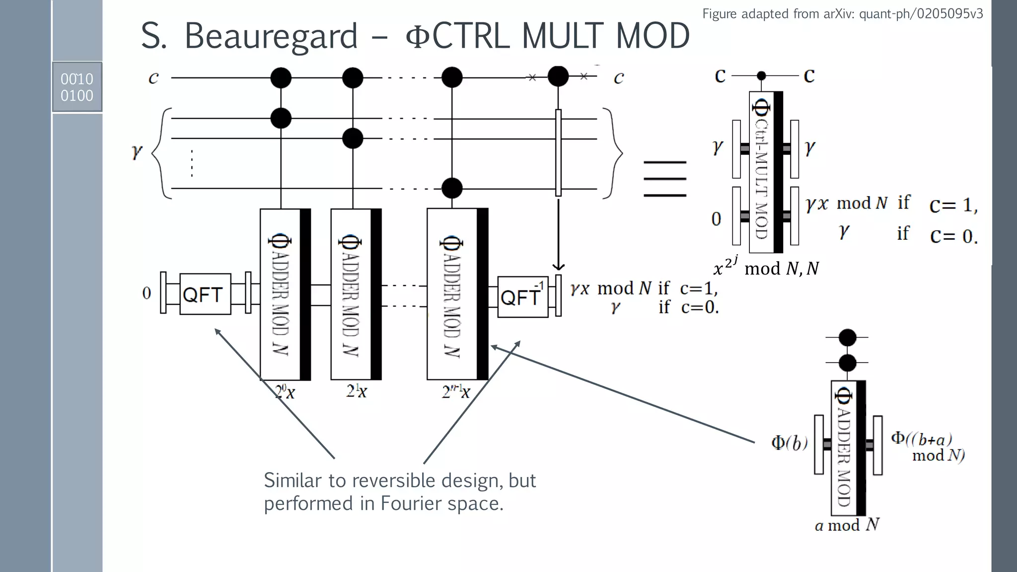
21. Quantum ADDER MOD Gate
0001
0101
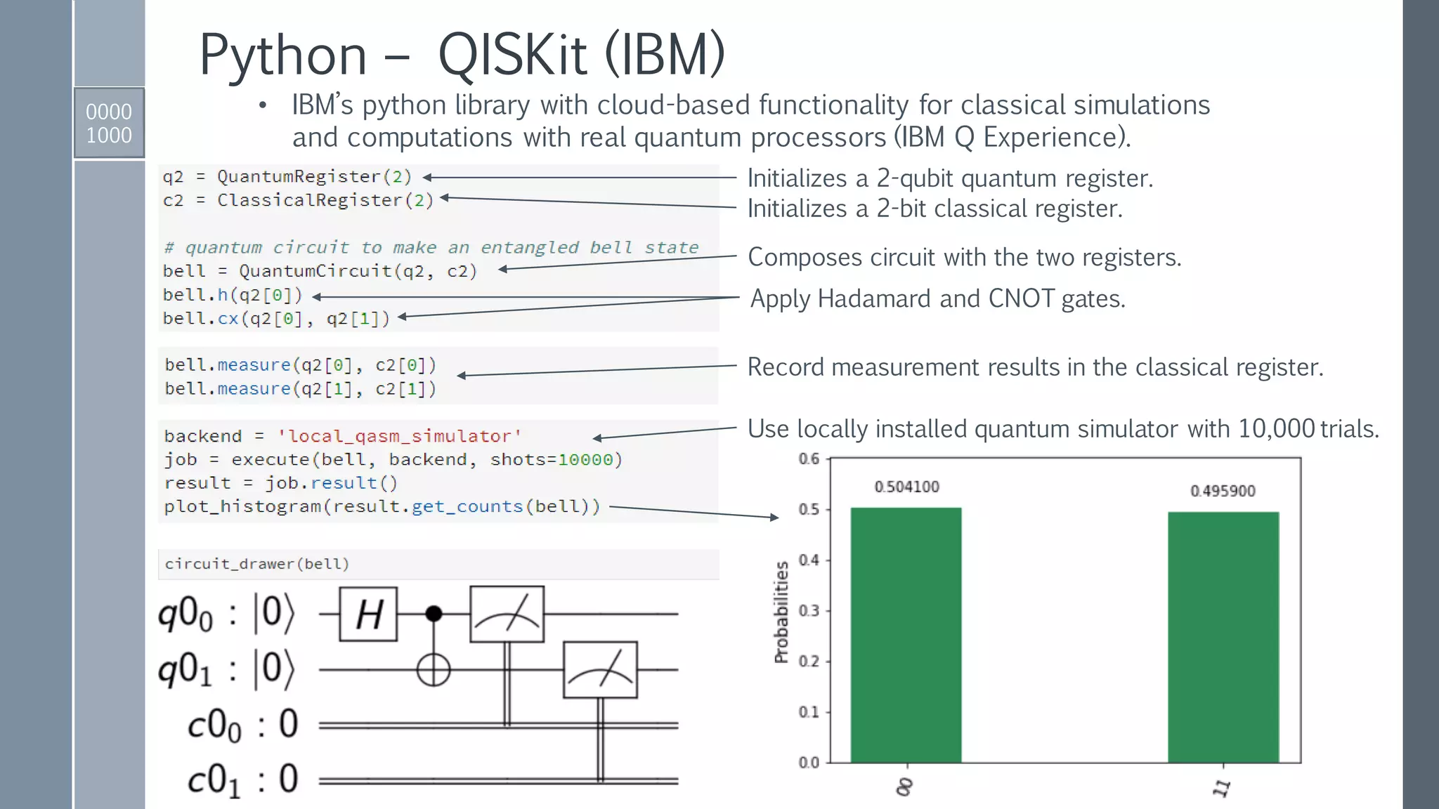
IBM QISKit implementation
ADDER gate to perform
𝑎, 𝑏 → |𝑎, 𝑎 + 𝑏⟩.
Reversed ADDER gate to perform:
𝑁, (𝑎 + 𝑏) → |𝑁,(𝑎 + 𝑏) − 𝑁⟩ if 𝑁 < 𝑎 + 𝑏,
𝑁, (𝑎 + 𝑏) → |𝑁, 2 𝑛+1−[𝑁 − 𝑎 + 𝑏 ]⟩ if 𝑁 > 𝑎 + 𝑏.
Conditionally set 𝑁-register to zero
if 𝑁 < 𝑎 + 𝑏 using MSB as control.
Conditionally add
either 0 or 𝑁 to
second register.
Conditionally
restore 𝑁-register.
Reversed
modules to
reset auxiliary.

22. Level Schematic
0001
0110
Register 1
Register 2
Auxiliary
Registers
|𝑘⟩ |𝑘⟩
|0⟩
|0⟩ |0⟩
Modules dependent
on Register 1 state
|𝑥 𝑘
mod 𝑁⟩

23. Strategy for 𝑘 0 → 𝑘 |𝑥 𝑘 mod 𝑁⟩:
Modular Exponentiation from Controlled Modular Multiplication0001
0111
We wish to implement 𝑓 𝑘 = 𝑥 𝑘 mod 𝑁 in Register 2.
• 𝑘 is the integer state of Register 1.
• 𝑥 is the known seed value.
• 𝑁 is the number we wish to factor.
Note that we can decompose 𝑓(𝑘) into 𝑡 multiplications using 𝑘’s binary representation :
= … 𝑥20 𝑘0 mod 𝑁 mod 𝑁 ⋅ 𝑥21 𝑘1 mod 𝑁 mod 𝑁 ⋅ … ⋅ 𝑥2 𝑡 𝑘 𝑡−1 mod 𝑁 mod 𝑁
𝑓 𝑘 = ෑ
𝑗=0
𝑡−1
𝑥2 𝑗 𝑘 𝑗 mod 𝑁 | mod 𝑁
𝑓 𝑘 = 𝑥20 𝑘0+21 𝑘1+⋯+2 𝑡−1 𝑘 𝑡−1 mod 𝑁
(evaluate mod 𝑁 after each multiplication)
𝑘 = 20
𝑘0 + 21
𝑘1 + ⋯ + 2 𝑡−1
𝑘 𝑡−1, so
𝑡 repeated multiplications with evaluation mod 𝑁
= … 𝑥20 𝑘0 mod 𝑁 ⋅ 𝑥21 𝑘1 mod 𝑁 ⋅ … ⋅ 𝑥2 𝑡−1 𝑘 𝑡−1 mod 𝑁

24. Strategy for 𝑘 0 → 𝑘 |𝑥 𝑘 mod 𝑁⟩:
Controlled Modular Multiplication from repeated Modular Addition0001
1000
From the previous slide we have:
Our goal is to now construct a controlled-multiplication gate
that takes some input 𝛾 → (𝛾 ⋅ 𝑥2 𝑗 𝑘 𝑗) mod 𝑁 for repeated use.
(𝛾 < 𝑁 will be the output from the previous multiplication gate).
Note that we can decompose 𝑥2 𝑗 𝑘 𝑗 into 𝑛 additions using the binary expansion of 𝑥2 𝑗 𝑘 𝑗:
𝑥2 𝑗 𝑘 𝑗 = 20
𝑥2 𝑗
0
+ 21
𝑥2 𝑗
1
+ ⋯ + 2 𝑡−1
𝑥2 𝑗
𝑡−1
𝑘 𝑗
= ෍
𝑖=0
𝑡−1
2𝑖 𝑥2 𝑗
𝑖
𝑘 𝑗
= ቊ 𝑥2 𝑗
1
if 𝑘𝑗 = 1,
if 𝑘𝑗 = 0.
if 𝑘𝑗 = 1,
if 𝑘𝑗 = 0.
Need our CTRL MULT MOD circuit to perform 𝑛 repeated summations with
evaluation mod 𝑁 if 𝑘𝑗 = 1, and to conditionally load 2 𝑚
𝑥2 𝑗
mod 𝑁 in the first
register of the appropriate ADDER MOD component if 𝑘𝑗 ∧ 𝛾 𝑚 = 1.
𝑓 𝑘 = ෑ
𝑗=0
𝑡−1
𝑥2 𝑗 𝑘 𝑗 mod 𝑁 | mod 𝑁
𝛾𝑥2 𝑗 𝑘 𝑗 mod 𝑁
෍
𝑚=0
𝑛−1
2 𝑚 𝛾 𝑚 𝑥2 𝑗
mod 𝑁 | mod 𝑁
𝛾

25. 0001
1001
Vedral et. al. – Quantum CTRL MULT MOD Gate
Conditionally load first
register with classically
computed 2 𝑚 𝑥2 𝑗
mod 𝑁.
Unload first register
immediately after gate
action and conditionally
reload with next value.
Copy 1st register to
output of 2nd register
if 𝑘𝑗 = 0.
Figure adapted from arXiv: quant-ph/9511018v1
𝑥2 𝑗
mod 𝑁, 𝑁

26. 0001
1010
Vedral et. al. – Quantum CTRL MULT MOD Gate
Figure adapted from arXiv: quant-ph/9511018v1
𝑥2 𝑗
mod 𝑁, 𝑁
Ex) let 𝑘𝑗 = 1:
1st register loaded with 20 𝛾0 𝑥2 𝑗
mod 𝑁.
2nd register outputs 0 + 20 𝛾0 𝑥2 𝑗
mod 𝑁 mod 𝑁.
1st register unloaded.
1st register reloaded with 21 𝛾1 𝑥2 𝑗
mod 𝑁.
2nd register outputs 0 + 20
𝛾0 𝑥2 𝑗
mod 𝑁 mod 𝑁 + 𝛾121
𝑥2 𝑗
mod 𝑁 mod 𝑁.
෍
𝑚=0
𝑛−1
2 𝑚 𝛾 𝑚 𝑥2 𝑗
| mod 𝑁 = 𝛾𝑥2 𝑗
mod 𝑁

27. 0001
1011
Figure adapted from arXiv: quant-ph/9511018v1
Vedral et. al. – Quantum EXP MOD Gate
Set input state of
Register 2 to |1⟩ so
output of first gate
is 𝑥 mod 𝑁 or 1.
Swap output registers and run
reverse CTRL MULT MOD gate that
implements modular multiplicative
inverse of previous gate’s action.
This sets the next gate’s secondary
input to 0.
𝑥, 𝑁

28. 0001
1100
Figure adapted from arXiv: quant-ph/9511018v1
Vedral et. al. – Quantum EXP MOD Gate
= 𝑥 𝑘
mod 𝑁Ex) let 𝑘0 ∧ 𝑘1 ∧ 𝑘2 = 1:
1st CTRL MULT MOD gate outputs 1 𝑥 mod 𝑁 . Output swapped to 𝑥 mod 𝑁 1 .
2nd CTRL MULT MOD (reversed) gate outputs 𝑥 mod 𝑁 |0⟩.
3rd CTRL MULT MOD gate outputs 𝑥 mod 𝑁 | 𝑥 mod 𝑁 ⋅ 𝑥2 mod 𝑁 mod 𝑁⟩. Output swapped.
4th CTRL MULT MOD (reversed) gate outputs 𝑥 mod 𝑁 ⋅ 𝑥2
mod 𝑁 mod 𝑁 |0⟩.
5th CTRL MULT MOD gate outputs:
𝑥 mod 𝑁 ⋅ 𝑥2
mod 𝑁 mod 𝑁 | 𝑥 mod 𝑁 ⋅ 𝑥2
mod 𝑁 mod 𝑁 ⋅ 𝑥4
mod 𝑁 mod 𝑁⟩.
𝑓 𝑘 = ෑ
𝑗=0
𝑡−1
𝑥2 𝑗 𝑘 𝑗 mod 𝑁 | mod 𝑁
𝑥, 𝑁

29. Qubit Requirement Analysis
0001
1101 Register 1
Register 2
Auxiliary
Registers
Let 𝑛 = log2 𝑁 .
Largest value 𝑘 relevant
for Shor’s Algorithm can
be as large as 𝑁2
.
Need 𝑡 ≥ 2𝑛 qubits in
Register 1, and 𝑛 qubits to
store result of 𝑥 𝑘 mod 𝑁 in
Register 2.
ADDER gate requires an
extra 𝑛 − 1 -qubit
temporary register for
carries, and 1 temporary
qubit to carry the MSB.
ADDER MOD gate requires
an extra 𝑛-qubit register to
store 𝑁, and 1 temporary
qubit for overflow control.
CTRL MULT MOD gate
requires an extra 𝑛-qubit
register to conditionally
load classically
computed values.
EXP MOD gate requires
an extra 𝑛-qubit register
to facilitate resets with
modular inverses
𝟐𝒏 qubits
𝒏 qubits
𝟒𝒏 + 𝟏
qubits
Network needs a total of 𝟕𝒏 + 𝟏 qubits to factor an 𝒏-bit number,
but can be reduced with some modifications (e.g. classical register
+ single qubit to keep track of entanglement in MOD ADDER).

30. 3. Fourier Space Improvements
0001
1110
And other optimizations to Draper’s reversible design

31. Fourier version gate set
0001
1111
Pauli X Gate Controlled-NOT Gate Toffoli Gate
Conditional Phase Shift Gate
• Similar design to classical-based
reversible circuits, with exception of
ADDER and ADDER MOD gates.
• Requires fewer qubits overall, but
also needs more gates to
implement additional Quantum
Fourier Transforms.

32. 0010
0000
QFT revisited
𝑏
1
2 𝑛
෍
𝑧=0
2 𝑛−1
exp
2𝜋𝑖𝑏𝑧
2 𝑡
𝑧 ,
𝑈 𝑄𝐹𝑇
Recall that the QFT of an integer state |𝑏⟩ on 𝑛 qubits is given by:
which can be factored as:
1
2 𝑛
෍
𝑧=0
2 𝑛−1
exp
2𝜋𝑖𝑏𝑧
2 𝑛 𝑧 = ໆ
𝑧=0
𝑛−1
1
2
0 + exp
2𝜋𝑖𝑏
2 𝑧+1 |1⟩ ,
= ໆ
𝑧=0
𝑛−1
1
2
0 + exp 2𝜋𝑖(0. 𝑏 𝑧 … 𝑏0 |1⟩
|𝜙 𝑏 ⟩ = ໆ
𝑧=0
𝑛−1
|𝜙 𝑧(𝑏)⟩.
Each |𝜙 𝑧 𝑏 ⟩ contains
the bottom 𝑧 bits of 𝑏.
ໆ
𝑧=0
𝑛−1
1
2
0 + exp 2𝜋𝑖(0. 𝑏 𝑧 … 𝑏0 + 𝟎. 𝒂 𝒛 … 𝒂 𝟎 |1⟩ = |𝜙 𝑏 + 𝑎 ⟩.
Want an ADDER circuit that performs Fourier space rotations controlled by bits of 𝑎:

33. 0010
0001
T. Draper – ΦADDER
Figure adapted from arXiv: quant-ph/0008033v1
Input 𝑛 qubits
representing a
number 𝑎.
Input 𝑛 qubits
representing
𝜙 𝑏 , the QFT
of a number 𝑏.
Output leaves 𝑎 unchanged,
but bottom register contains
the QFT of (𝑎 + 𝑏).
Conditional phase shift gates
Circumvents need for
𝒏-qubit carry register.
Extra qubit in
answer register
for overflow

34. 0010
0010
T. Draper – ΦADDER
Figure adapted from arXiv: quant-ph/0008033v1
=
1
2
0 + exp 2𝜋𝑖(0. 𝑏 𝑧 … 𝑏0 |1⟩
1
2
0 + exp 2𝜋𝑖(0. 𝑏 𝑧 … 𝑏0 + 0. 𝑎 𝑧 |1⟩
1
2
0 + exp 2𝜋𝑖(0. 𝑏 𝑧 … 𝑏0 + 0. 𝑎 𝑧 𝑎 𝑧−1 |1⟩
1
2
0 + exp 2𝜋𝑖(0. 𝑏 𝑧 … 𝑏0 + 0. 𝑎 𝑧 … 𝑎0 |1⟩
|𝜙 𝑧(𝑏)⟩
(𝑎 𝑧 rotation)
(𝑎 𝑧−1 rotation)
(𝑎0 rotation)
⋮
𝜙 𝑧 𝑏 + 𝑎 =
Ex)

35. 0010
0011
S. Beauregard – ΦADDER MOD
Figure adapted from arXiv: quant-ph/0205095v3
Similar design to classical-based reversible
ADDER MOD, but with extra gate
requirements to construct intermediary
QFTs, which are necessary to be able to
use the MSB to check if 𝑎 + 𝑏 < 𝑁.
Can classically pre-compute
total phase shifts for each
qubit to eliminate a register.

36. 00`10
0100
S. Beauregard – ΦCTRL MULT MOD
Similar to reversible design, but
performed in Fourier space.
Figure adapted from arXiv: quant-ph/0205095v3
𝑥2 𝑗
mod 𝑁, 𝑁

37. 0010
0101
S. Beauregard – One-CTRL Qubit Trick
Figure adapted from arXiv: quant-ph/0205095v3
Uses 1 qubit to control
modular exponentiation
instead of 2𝑛 qubits.
Measurement results determine
which transformation to apply
prior to the next measurement
(conditionally apply 𝑋 gates).
𝑅 gates implement QFT
conditionally on previous
measurement result.
Measurements yield
desired output of
Shor’s Algorithm.

38. Qubit Requirement Analysis
0001
0110 Controlling qubit
Main Register
Auxiliary
Registers
Let 𝑛 = log2 𝑁 .
𝛷ADDER gate requires 1
extra qubit to prevent
overflow.
𝛷ADDER MOD gate
requires 1 extra
control qubit.
𝛷CTRL MULT MOD gate requires an extra
𝑛-qubit register to conditionally load
classically computed values, which can
also be repurposed to facilitate swaps.
𝟏 qubit
𝒏 qubits
𝒏 + 𝟐
qubits
Network needs a total of 𝟐𝒏 + 𝟑 qubits to factor an 𝒏-bit number.

39. Appendix
Shor’s Algorithm Detailed Description
0010
0111

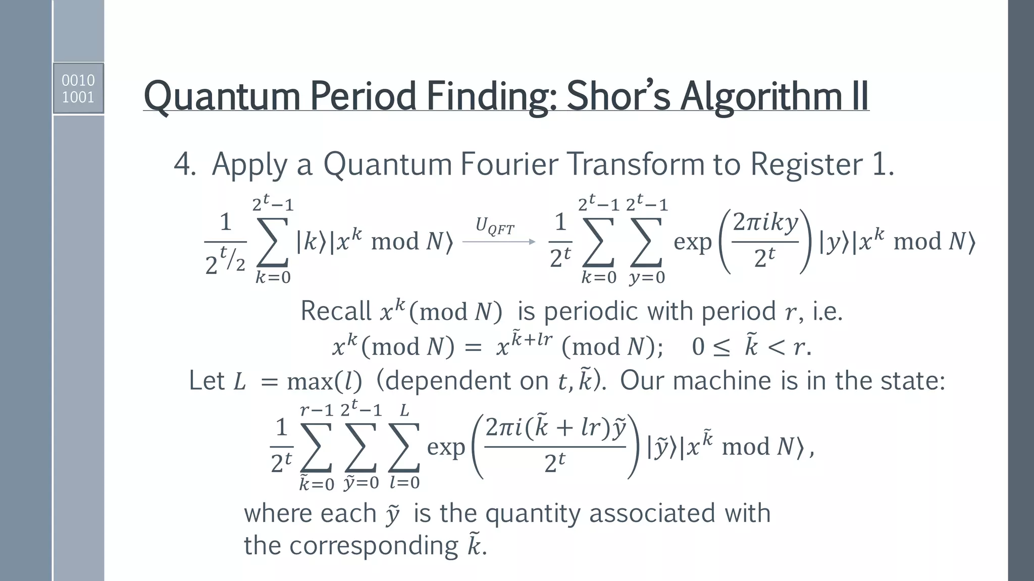
40. Quantum Period Finding: Shor’s Algorithm I
1. Initialize registers to zero-position.
00 … 00 00 …00 = 0 |0⟩
|Register 1⟩ |Register 2⟩
2. Apply Hadamard gates to the 𝑡 qubits in Register 1.
0 0
1
2 ൗ𝑡
2
෍
𝑘=0
2 𝑡−1
𝑘 |0⟩
𝐻⊗𝑡
3. Apply a quantum function that performs the map:
𝑈𝑓1
2 ൗ𝑡
2
෍
𝑘=0
2 𝑡−1
𝑘 0
1
2 ൗ𝑡
2
෍
𝑘=0
2 𝑡−1
𝑘 |𝑥 𝑘
mod 𝑁⟩
0010
1000
𝑡 qubits in Register 1 to encode
integers [0, …, 2 𝑡
− 1] in binary;
𝑡 larger than 2𝑛 = 2 log2 𝑁 .

41. Quantum Period Finding: Shor’s Algorithm II
4. Apply a Quantum Fourier Transform to Register 1.
1
2 ൗ𝑡
2
෍
𝑘=0
2 𝑡−1
𝑘 |𝑥 𝑘
mod 𝑁⟩
1
2 𝑡 ෍
𝑘=0
2 𝑡−1
෍
𝑦=0
2 𝑡−1
exp
2𝜋𝑖𝑘𝑦
2 𝑡
𝑦 |𝑥 𝑘
mod 𝑁⟩
𝑈 𝑄𝐹𝑇
Recall 𝑥 𝑘
mod 𝑁 is periodic with period 𝑟, i.e.
𝑥 𝑘
mod 𝑁 = 𝑥
෨𝑘+𝑙𝑟
mod 𝑁 ; 0 ≤ ෨𝑘 < 𝑟.
1
2 𝑡 ෍
෨𝑘=0
𝑟−1
෍
෤𝑦=0
2 𝑡−1
෍
𝑙=0
𝐿
exp
2𝜋𝑖(෨𝑘 + 𝑙𝑟)෤𝑦
2 𝑡
෤𝑦 |𝑥
෨𝑘
mod 𝑁⟩ ,
where each ෤𝑦 is the quantity associated with
the corresponding ෨𝑘.
Let 𝐿 = max 𝑙 (dependent on 𝑡, ෨𝑘). Our machine is in the state:
0010
1001

42. Quantum Period Finding: Shor’s Algorithm III
𝜓 =
1
2 𝑡 ෍
෨𝑘=0
𝑟−1
෍
෤𝑦=0
2 𝑡−1
෍
𝑙=0
𝐿
exp
2𝜋𝑖(෨𝑘 + 𝑙𝑟)෤𝑦
2 𝑡
෤𝑦 |𝑥
෨𝑘
mod 𝑁⟩
Observation: Periodic in 𝑟 for any ෨𝑘.
Information of period was loaded into amplitudes when we applied the QFT.
5. Perform measurement of Register 1.
For any particular ෤𝑦 |𝑥
෨𝑘
mod 𝑁⟩:
𝐴 ෤𝑦, ෨𝑘, 𝑟 =
1
2 𝑡 ෍
𝑙=0
𝐿
exp
2𝜋𝑖(෨𝑘 + 𝑙𝑟)෤𝑦
2 𝑡
𝑃 ෤𝑦, ෨𝑘, 𝑟 =
1
2 𝑡
2
෍
𝑙=0
𝐿
exp
2𝜋𝑖𝑙𝑟෤𝑦
2 𝑡
2
Very weak dependence on ෨𝑘
(𝐿 = max 𝑙 may differ by 1 with ෨𝑘)
Probability of observing a particular ෤𝑦
is approximately the same for all ෨𝑘.
0010
1010

43. Quantum Period Finding: Shor’s Algorithm IV
𝑃 ෤𝑦, ෨𝑘, 𝑟 =
1
2 𝑡
2
෍
𝑙=0
𝐿
exp
2𝜋𝑖𝑙𝑟෤𝑦
2 𝑡
2
6. Classical post processing.
Observation: probability peaks at
𝐿+1
2 𝑡
2
when
𝑟 ෤𝑦
2 𝑡 ∈ ℤ.
Locations of probability peaks (as function of ෤𝑦) encode 𝑟 as an
integer multiple of
2 𝑡
෤𝑦
. Since 𝑡 is set by the user and each ෤𝑦 is known
from measurement, we can perform multiple measurements and
extract 𝑟 using efficient classical techniques.
e.g. use continued fractions to find
𝛽
𝑟
satisfying
෤𝑦
2 𝑡 −
𝛽
𝑟
≤
1
2 𝑡+1, 𝛽 ∈ ℤ.
0010
1011

44. Recall that the simple continued fraction expansion a real number 𝑅 is of the form:
𝑎0 +
1
𝑎1 +
1
𝑎2 +
1
…
Recall that convergents of the continued fraction are rational approximations of 𝑅.
Shor’s idea: Use the convergents of
෤𝑦
2 𝑡
to obtain
𝛽
𝑟
in lowest terms,
such that
෤𝑦
2 𝑡 −
𝛽
𝑟
≤
1
2 𝑡+1 is satisfied (intuitively,
෤𝑦
2 𝑡 =
𝛽
𝑟
up to some
small error outside the possible resolution of the system).
Quantum Period Finding: Shor’s Algorithm V
The 𝑗th convergent
𝛽𝑗
𝑟 𝑗
of a continued fraction expansion is given recursively by:
The first two convergents are:
𝛽0
𝑟0
=
𝑎0
1
,
𝛽1
𝑟1
=
𝑎1 𝑎0 + 1
𝑎1
𝛽𝑗
𝑟𝑗
=
𝑎 𝑛 𝛽 𝑛−1 + 𝛽 𝑛−2
𝑎 𝑛 𝑟𝑛−1 + 𝑟𝑛−2
0010
1100

45. Appendix
Shor’s Algorithm Example: Factoring N = 21
0010
1101

46. Quantum Period Finding Example: 𝑵 = 𝟐𝟏
Using 𝑡 = 7 qubits in each register:
𝐻⊗7
0 0
1
27
෍
𝑘=0
27−1
𝑘 |0⟩
2. Apply Hadamard gates to qubits in Register 1.
1. Initialize.
=
1
27
0 + 1 + ⋯+ 126 + |127⟩ |0⟩
0 0 = 0000000 0000000
0000000 + 0000001 + ⋯ + |1111111⟩ |0000000⟩
0010
1110
(ideally for good precision, should use at least log2 21 = 5
qubits in Register 2 and 𝑡 > 2 log2 21 = 2𝑛 = 10 in Register 1).

47. Quantum Period Finding Example: 𝑵 = 𝟐𝟏
1
27
෍
𝑘=0
27−1
𝑘 0
1
27
෍
𝑘=0
27−1
𝑘 |5 𝑘
mod 21⟩
𝑈𝑓
=
1
27
0 50
mod 21 + 1 51
mod 21 + ⋯+
126 |5126
mod 21⟩ + |127⟩|5127
mod 21⟩
(
)
=
1
27
0 1 + 1 5 + 2 4 + 3 20 + 4 16 + 5 17 +(
6 1 + 7 5 + 8 4 + 9 20 + 10 16 + 11 17 +
… + |123⟩|4⟩ + |124⟩|20⟩ + 125 17 + 126 1 + 127 5 )
𝑟 = 6, but this information is still hidden from the user
3. Apply the quantum function with (randomly chosen) 𝑥 = 5.
0010
1111

48. Quantum Period Finding Example: 𝑵 = 𝟐𝟏
1
27
෍
𝑘=0
27−1
𝑘 |5 𝑘
mod 21⟩
1
27 ෍
𝑘=0
27−1
෍
𝑦=0
27−1
exp
2𝜋𝑖𝑘𝑦
27
𝑦 |5 𝑘
mod 21⟩
4. Apply a Quantum Fourier Transform to Register 1.
𝑈 𝑄𝐹𝑇
1
27 ෍
෨𝑘=0
6−1
෍
෤𝑦=0
27−1
෍
𝑙=0
𝐿
exp
2𝜋𝑖(෨𝑘 + 6𝑙)෤𝑦
27
෤𝑦 |5
෨𝑘
mod 21⟩
Information of period encoded in amplitudes
Hidden information (for classical analysis) | 𝑟 = 6, 𝑘 = ෩𝑘 + 𝑙𝑟.
෩𝒌 0 1 2 3 4 5
𝟓
෩𝒌
𝐦𝐨𝐝 𝟐𝟏 1 5 4 20 16 17
𝑳 = 𝐦𝐚𝐱(𝒍) 21 21 20 20 20 20
0011
0000

49. Quantum Period Finding Example: 𝑵 = 𝟐𝟏
5. Perform measurement of Register 1.
Suppose we want the probability observing some particular ෤𝑦 |5
෨𝑘
mod 21⟩,
e.g. probability of observing ෤𝑦 20 (⇔ ෨𝑘 = 4 since 54 (mod 21) = 20).
𝑃 ෤𝑦, ෨𝑘, 𝑟 → 𝑃 ෤𝑦, 4, 6 =
1
27
2
෍
𝑙=0
20
exp
2𝜋𝑖𝑙6෤𝑦
27
2
Can analytically obtain the probability spectrum as a function of only ෤𝑦 (and
hidden 𝑟) by summing over all unique residues ෨𝑘 of 𝑘 mod 𝑟.
Explicit formula is useless without prior knowledge of 𝑟,
but spectrum can be used to verify experimental results.
𝑃 ෤𝑦 =
1
27
2
2 ෍
𝑙=0
21
exp
2𝜋𝑖𝑙6෤𝑦
27
2
+ 4 ෍
𝑙=0
20
exp
2𝜋𝑖𝑙6෤𝑦
27
2
0011
0001

50. Quantum Period Finding Example: 𝑵 = 𝟐𝟏
𝑃 ෤𝑦 =
1
27
2
2 ෍
𝑙=0
21
exp
2𝜋𝑖𝑙6෤𝑦
27
2
+ 4 ෍
𝑙=0
20
exp
2𝜋𝑖𝑙6෤𝑦
27
2
෤𝑦 = 21 ෤𝑦 = 43
෤𝑦 = 64
෤𝑦 = 85 ෤𝑦 = 107
Spectrum explicit equation (𝑁 = 21, 𝑟 = 6):
Probability spectrum:
0010
0010

51. Quantum Period Finding Example: 𝑵 = 𝟐𝟏
0011
0011
6. Classical post processing using continued fractions.
Suppose we measure ෤𝑦 = 107 in Register 1.
107
128
−
𝛽
𝑟
≤
1
256
Goal: find
𝛽
𝑟
such that
0 +
1
1 +
1
5 +
1
10 +
1
2
107
128
=
𝛽0
𝑟0
=
𝑎0
1
,
𝛽1
𝑟1
=
𝑎1 𝑎0 + 1
𝑎1
,
𝛽𝑗
𝑟𝑗
=
𝑎 𝑛 𝛽 𝑛−1 + 𝛽 𝑛−2
𝑎 𝑛 𝑟𝑛−1 + 𝑟𝑛−2
𝛽0
𝑟0
=
0
1
,
𝛽1
𝑟1
=
1 ⋅ 0 + 1
1
,
𝛽2
𝑟2
=
5 ⋅ 1 + 0
5 ⋅ 1 + 1
=
5
6
𝑟 = 6
Check that 𝑥 Τ𝑟
2 ≢ ±1 mod 𝑁
Choose new 𝑥 and repeat steps to find period. (𝑥 = 11 , 𝑟 = 6).
𝑝 = gcd 𝑥 Τ𝑟
2 − 1, 𝑁
𝑞 = gcd 𝑥 Τ𝑟
2 + 1, 𝑁
𝑝 = gcd 11 Τ6
2 − 1, 21
𝑞 = gcd 11 Τ6
2 + 1, 21
𝑝 = 7
𝑞 = 3
53 ≡ −1 (mod 21)

52. Appendix
Why care about integer factorization?
Integer factorization in RSA context
0011
0100

53. RSA Cryptosystem
- Wants to send message 𝑀 to Bob - Uses RSA encryption scheme
- Wants to learn 𝑀
Alice Bob
Eve
• RSA (Rivest–Shamir–Adleman) is a popular modern data encryption protocol.
• Security boils down to the difficulty of factoring the product of two large primes.
0011
0101

54. RSA Scheme: KeyGen Step (Bob)
1. Choose prime numbers 𝑝 and 𝑞 which are roughly the same bit-size.
2. Compute N = 𝑝 ⋅ 𝑞. (public)
3. Compute 𝜆 𝑁 = lcm 𝑝 − 1, 𝑞 − 1 =
𝑝−1 ⋅(𝑞−1)
gcd(𝑝−1,𝑞−1)
. (private)
4. Choose integer e; 1 < 𝑒 < 𝜆 𝑁 , gcd 𝑒, 𝜆 𝑁 = 1. (public)
5. Compute 𝒅 = 𝑒−1
(mod 𝜆(𝑁)). (private)
Public Key Pair
(𝑁, 𝒆)
Sent to Alice (+ World)
Private Key Pair
(𝑁, 𝒅)
Kept by Bob
0011
0110

55. RSA Scheme: Encryption Step (Alice)
1. Convert 𝑀 (plaintext) to 𝑚 (integer) via padding scheme.
2. Compute 𝑐 = 𝑚 𝑒
(mod N).
3. Transmit 𝑐 (ciphertext) to Bob.
RSA Scheme: Decryption Step (Bob)
1. Receive 𝑐 (ciphertext) from Alice.
2. Compute 𝑚 = 𝑐 𝑑
(mod 𝑁) = 𝑚 𝑒 𝑑
(mod 𝑁).
3. Recover 𝑀 (plaintext) from 𝑚 (integer) via padding scheme.
0011
0111

56. RSA Scheme: Example
𝑀 = ‘hi’
Public Info (Alice + World)
• (𝑁, 𝒆) = (4757, 𝟏𝟕)
Private Info (Bob)
• 𝑝 = 71, 𝑞 = 67 | (𝑁 = 4757)
• 𝜆 𝑁 = lcm 70, 66 = 2310
• gcd 𝒆, 𝜆 𝑁 = gcd 17, 2310 = 1.
• 𝒅 = 𝑒−1
mod 𝜆 𝑁 = 17−1
mod 2310 = 1223
• (𝑁, 𝒅) = (4757, 𝟏𝟐𝟐𝟑)
𝑚 = 89
𝑐 = 𝑚 𝑒
mod 𝑁
𝑐 = 8917
mod 4757
Alice Bob
𝑐 = 3978
(𝑁, 𝒆) = (4757, 𝟏𝟕) (𝑁, 𝒅) = (4757, 𝟏𝟐𝟐𝟑)
𝑚 = 39781223 (mod 4757)
𝑚 = 𝑐 𝑑 𝑚𝑜𝑑 𝑁
𝑚 = 89
𝑀 = ‘hi’
0011
1000

57. Eve
• Eve efficiently factors 𝑁 = 4757 into 71 ⋅ 67.
• Eve computes 𝜆 𝑁 = 𝑙𝑐𝑚 70, 66 = 2310.
• Eve computes 𝒅 = 𝒆−1 𝑚𝑜𝑑 𝜆 𝑁 .
• Eve intercepts 𝑐.
• Eve recovers 𝑀 using Bob’s procedure.
𝑀 = ‘hi’
𝑚 = 89
𝑐 = 𝑚 𝑒
mod 𝑁
𝑐 = 8917
mod 4757
Bob
𝑐 = 3978
(𝑁, 𝒆) = (4757, 𝟏𝟕) (𝑁, 𝒅) = (4757, 𝟏𝟐𝟐𝟑)
𝑚 = 39781223 (mod 4757)
𝑚 = 𝑐 𝑑 𝑚𝑜𝑑 𝑁
𝑚 = 89
𝑀 = ‘hi’
Alice
RSA Scheme: Example (Efficient Eve)
0011
1001