Downloaded 643 times
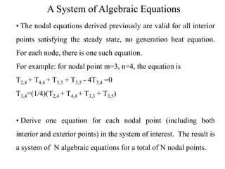
![Matrix Form
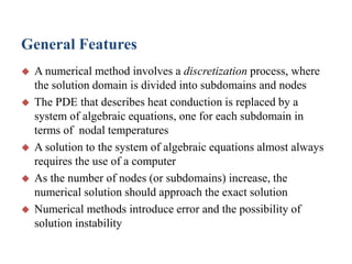
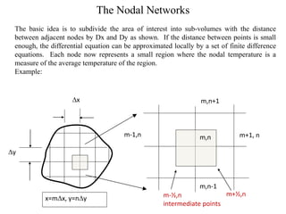
The system of equations:
a11T1 a12T2 a1N TN C1
a21T1 a22T2
a2 N TN C2
a N 1T1 a N 2T2
a NN TN CN
A total of N algebraic equations for the N nodal points and the system can be
expressed as a matrix formulation: [A][T]=[C]
a11 a12
a
a22
21
where A=
aN 1 aN 2
a1N
T1
C1
T
C
a2 N
, T 2 ,C 2
aNN
TN
C N ](https://image.slidesharecdn.com/numericalmethodsfor2-dheattransfer-140309114702-phpapp02/85/Numerical-methods-for-2-d-heat-transfer-13-320.jpg)
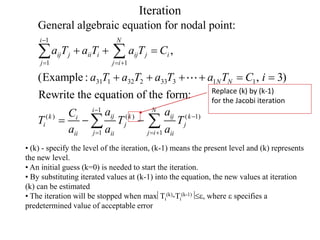
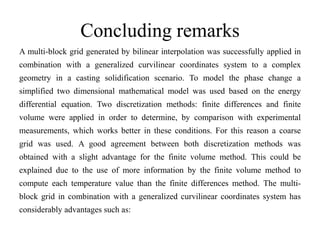
![Numerical Solutions
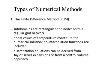
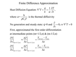
Matrix form: [A][T]=[C].
From linear algebra: [A]-1[A][T]=[A]-1[C], [T]=[A]-1[C]
where [A]-1 is the inverse of matrix [A]. [T] is the solution vector.
• Matrix inversion requires cumbersome numerical computations and is not efficient if
the order of the matrix is high (>10).
• For high order matrix, iterative methods are usually more efficient. The famous
Jacobi & Gauss-Seidel iteration methods will be introduced in the following.](https://image.slidesharecdn.com/numericalmethodsfor2-dheattransfer-140309114702-phpapp02/85/Numerical-methods-for-2-d-heat-transfer-14-320.jpg)
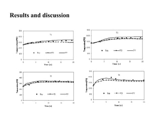


This document presents a numerical study comparing finite difference and finite volume methods for solving the heat transfer equation during solidification in a complex casting geometry. The study uses a multi-block grid with bilinear interpolation and generalized curvilinear coordinates. Results show good agreement between the two discretization methods, with a slight advantage for the finite volume method due to its use of more nodal information. The multi-block grid approach reduces computational time and allows complex geometries to be accurately modeled while overcoming issues at block interfaces.