Download to read offline
![ABSTRACT
FORTRAN is used as a numerical and scientific computing language. The main objective
of the lab work is to understand FORTRAN language using which we solve simple
numerical problems and compare different methodologies. Through this project we make
use of various functions of FORTRAN and solve a FDM simple heat equation problem
applying different conditions viz. Dirichlet and Von Neumann. The given problems are
solved analytically then built and compiled using a free integrated development
environment called CODE::BLOCKS [1] which is an open source platform for FORTRAN
and C.](https://image.slidesharecdn.com/lw2-dnm2019-penkulintinarasimhaprasad-200126084000/75/Projectwork-on-different-boundary-conditions-in-FDM-2-2048.jpg)
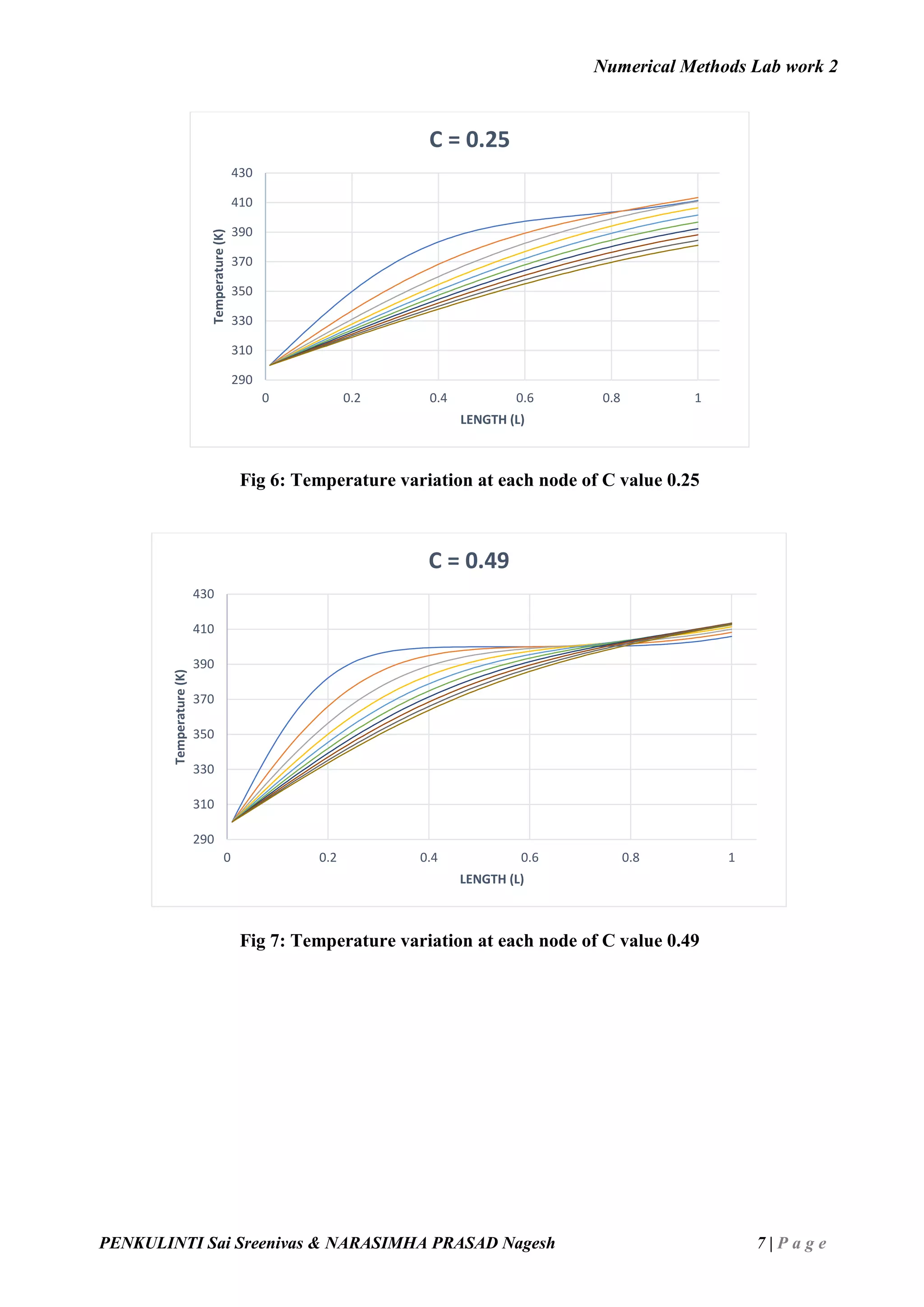
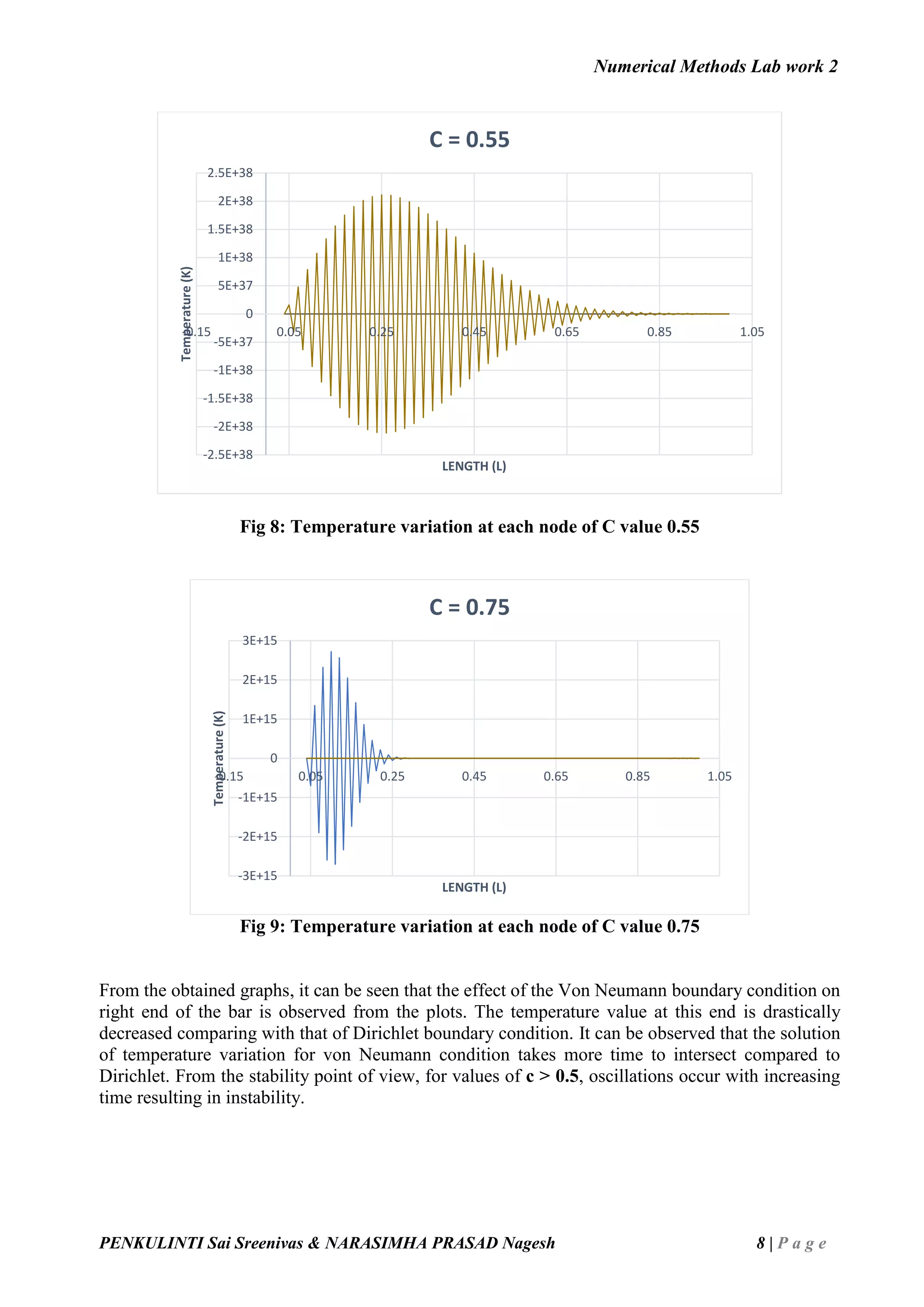
![Numerical Methods Lab work 2
PENKULINTI Sai Sreenivas & NARASIMHA PRASAD Nagesh 3 | P a g e
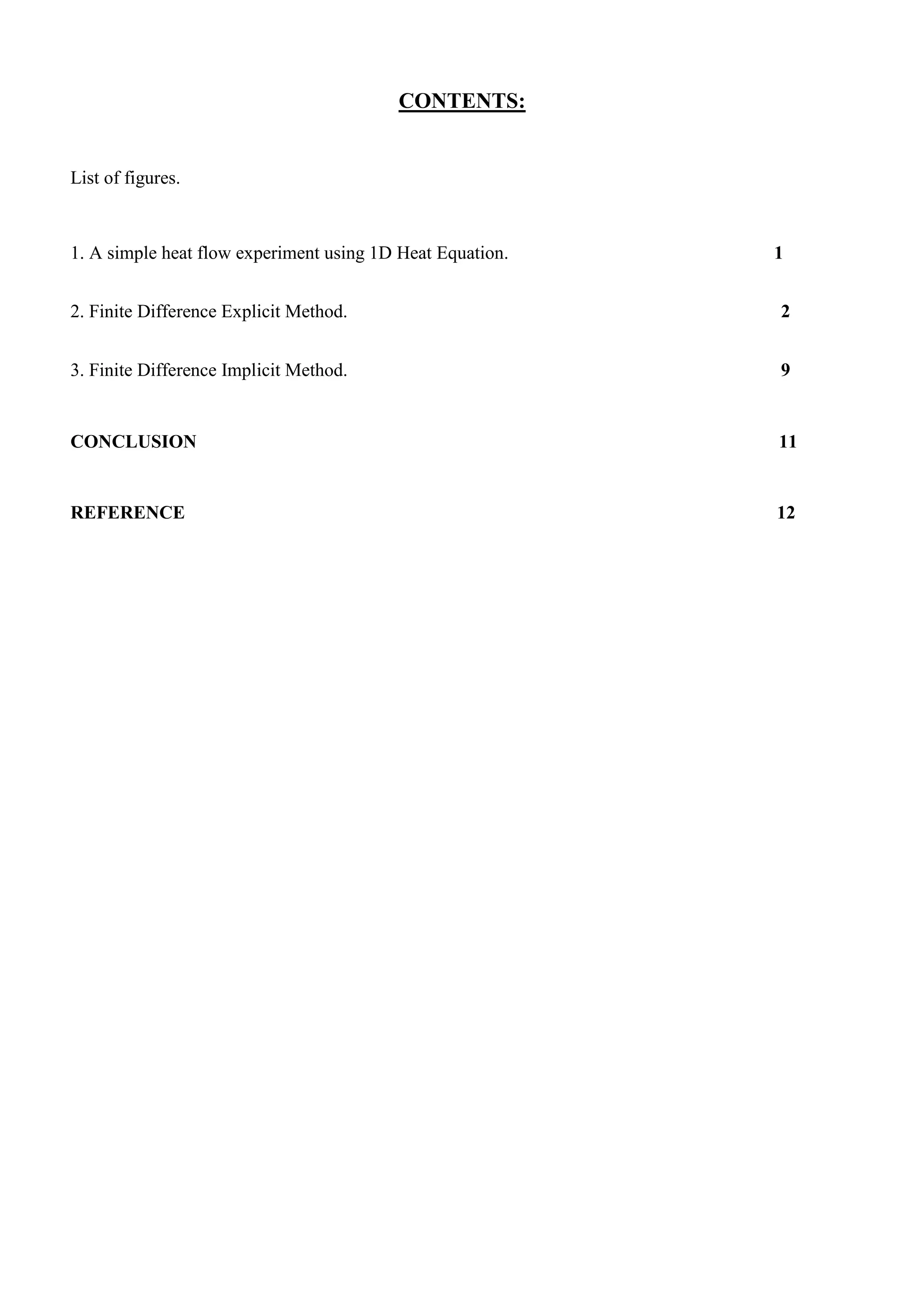
The initial condition is T(x, 1) = 400 indicating 𝑇𝑗
1
= 400
Applying the boundary conditions in the obtained equation 5 with j varying from 2 to N-1
𝑇𝑗
𝑘+1
= 𝑐𝑇𝑗−1
𝑘
+ (1 − 2𝑐)𝑇𝑗
𝑘
+ 𝑐𝑇𝑗+1
𝑘
The equation for the second node can be written as,
𝑇2
𝑘+1
= 𝑐𝑇1
𝑘
+ (1 − 2𝑐)𝑇2
𝑘
+ 𝑐𝑇3
𝑘
𝑇2
𝑘+1
= 300𝑐 + (1 − 2𝑐)𝑇2
𝑘
+ 𝑐𝑇3
𝑘
The equation for the last but one node can be written as,
𝑇 𝑁−1
𝑘+1
= 𝑐𝑇 𝑁−2
𝑘
+ (1 − 2𝑐)𝑇 𝑁−1
𝑘
+ 𝑐𝑇 𝑁
𝑘
𝑇 𝑁−1
𝑘+1
= 𝑐𝑇 𝑁−2
𝑘
+ (1 − 2𝑐)𝑇 𝑁−1
𝑘
+ 500𝑐
Writing the system of equations in the matrix form:
𝑻 𝒌+𝟏
= 𝑨𝑻 𝒌
+ 𝑩
(
𝑇1
𝑘+1
⋮
𝑇 𝑁
𝑘+1
) = [
1 − 2𝑐 𝑐 0
𝑐 ⋱ ⋱
0 ⋱ 1 − 2𝑐
] (
𝑇1
𝑘
⋮
𝑇 𝑁
𝑘
) + [
300
⋮
500
]
Here (1-2c) occupies the main diagonal and c the lower and upper diagonal. B is the boundary
condition matrix with only two entries at the extreme nodes and the other values are 0.
By applying the derived equation into program graphs for temperature values as function of time for
different length divisions can be obtained.](https://image.slidesharecdn.com/lw2-dnm2019-penkulintinarasimhaprasad-200126084000/75/Projectwork-on-different-boundary-conditions-in-FDM-7-2048.jpg)
![Numerical Methods Lab work 2
PENKULINTI Sai Sreenivas & NARASIMHA PRASAD Nagesh 10 | P a g e
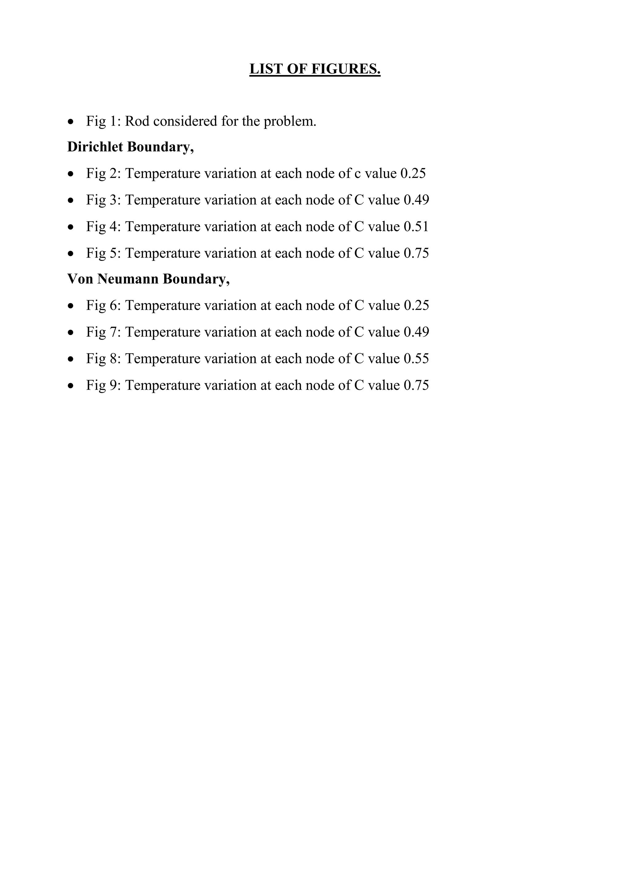
The equation for the last but one nod can be written as,
𝑇 𝑁−1
𝑘
= −𝑐𝑇 𝑁−1
𝑘+1
+ (1 + 2𝑐)𝑇 𝑁
𝑘+1
− 𝑐𝑇 𝑁+1
𝑘+1
This temperature is maintained at all times for this problem. The initial condition is same as the
previous one given by T(x, 1) = 400 indicating,
𝑇𝑗
1
= 400
Applying the boundary conditions in the obtained equation with j varying from 2 to N-1
𝑇𝑗
𝑘
= −𝑐𝑇𝑗−1
𝑘+1
+ (1 + 2𝑐)𝑇𝑗
𝑘+1
− 𝑐𝑇𝑗+1
𝑘+1
Writing the system of equation in the matrix form
𝐴. 𝑇 𝑘+1
= 𝑇 𝑘
+ 𝐵
[
1 + 2𝑐 −𝑐 0
−𝑐 ⋱ ⋱
0 ⋱ 1 + 2𝑐
] (
𝑇1
𝑘+1
⋮
𝑇 𝑁
𝑘+1
) = (
𝑇1
𝑘
⋮
𝑇 𝑁
𝑘
) + [
300
⋮
500
]
Where A is tridiagonal matrix with 1+2c as the main diagonal and -c as the lower and upper diagonal.
B is the boundary condition matrix with only two entries at the extreme nodes and the other values
being 0.](https://image.slidesharecdn.com/lw2-dnm2019-penkulintinarasimhaprasad-200126084000/75/Projectwork-on-different-boundary-conditions-in-FDM-14-2048.jpg)

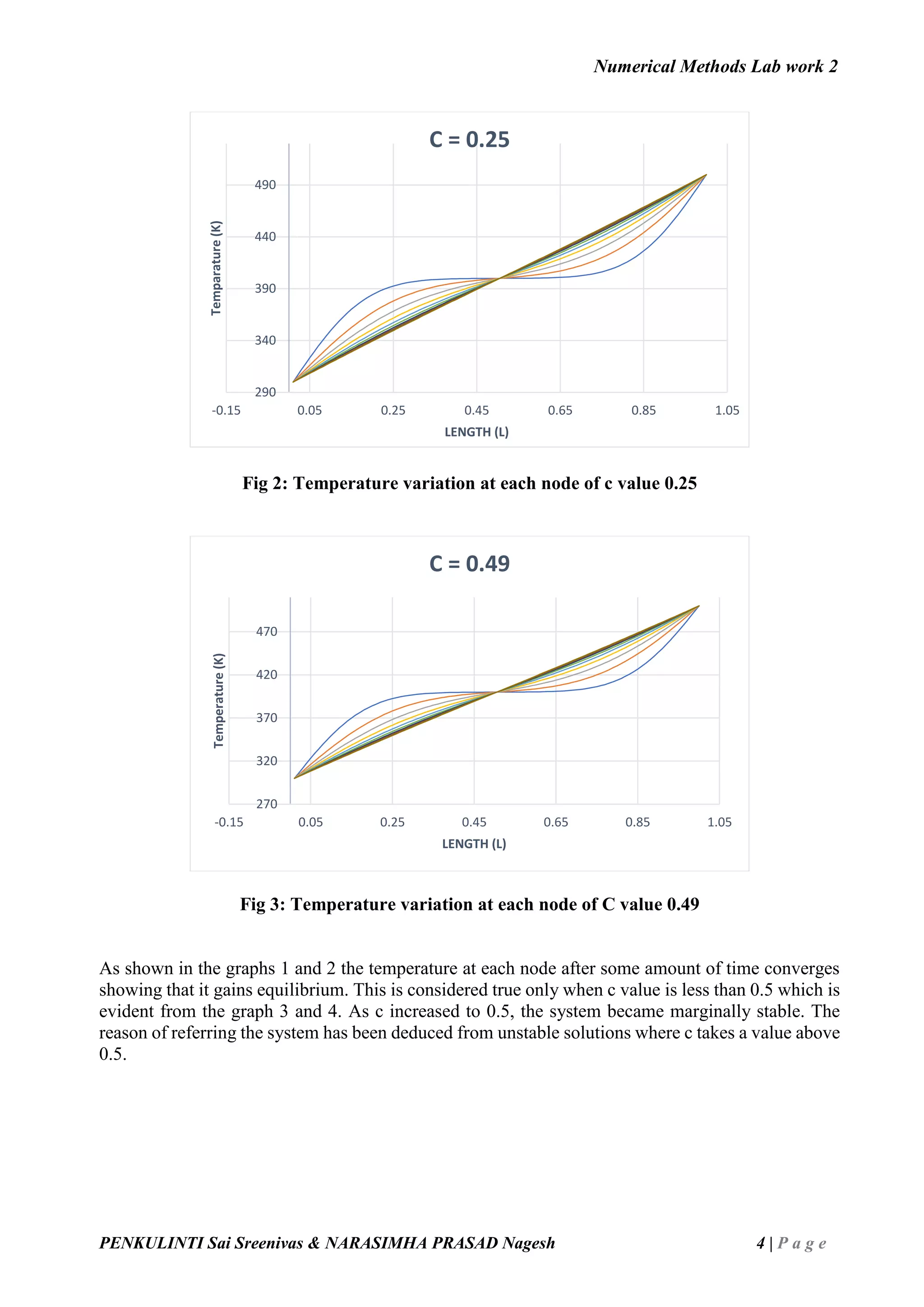
This document details a numerical methods lab work focused on using Fortran to solve a simple heat equation for a copper rod under two boundary conditions: Dirichlet and von Neumann. The lab involves applying finite difference methodologies to analyze temperature variations at different nodes of the rod over time, highlighting stability concerns with various values of the finite difference parameter 'c'. It concludes with insights gained from the project and references for further learning about Fortran.


