SlideShare a Scribd company logo
1 of 62
Download to read offline
A Comparison of Recent Trends of International
Marriages and Divorces in European Countries
Giampaolo LANZIERI
Statistical Office of the European Union (Eurostat)
Acknowledgements
I sincerely thank for their release of additional data and/or information the statistical
offices of: Albania, Andorra, Austria, Belarus, Belgium, Bosnia-Herzegovina, Bulgaria,
Croatia, Cyprus, Czech Republic, Denmark, Estonia, Finland, France, Germany,
Hungary, Iceland, Ireland, Latvia, Liechtenstein, Lithuania, Malta, Montenegro,
Moldova, Norway, Poland, Portugal, Romania, Russia, Serbia, Slovakia, Slovenia,
Spain, Switzerland, Turkey.
Disclaimer
This paper is released to inform interested parties about research work and to encourage
discussion. As this paper is solely a personal initiative of the author, the views
expressed are exclusively those of the author and do not necessarily represent the views
of the European Commission / Eurostat.
Date of last revision: August 2011
1
Abstract
Based on annual data by national/foreign citizenship from official statistics, the paper
analyses the latest trends of international and mixed marriages and divorces in a large
number of European countries. This provides as well a broad overview of the social
distances between nationals and foreigners across Europe in the first decade of the new
century, particularly relevant in a geographical area in which migration has become
the most important component of demographic change and it is expected to continue
playing an important role in the coming years. Further, for those countries belonging to
the European Union, the study takes into account the stocks of foreigners and compares
indicators based on mixed marriages to two datasets of indicators which are currently
proposed to the attention of policy-makers to measure the integration of the immigrants.
1. Introduction
In the last two decades, several European countries, especially those members of the
European Union (EU), have experienced important migratory inflows and others have
turned from sender to net receiving countries. Since 1992, migration has become the
most important component of population change in the EU (Lanzieri 2008), ensuring
the continuation of the population growth or attenuating its decline, role confirmed still
today (Marcu 2011). Considering the potential need of further immigration for an
ageing Europe and the contribution that migrants bring to the demographic change of
the host countries, the European societies are likely to become more and more
diversified (Lanzieri 2010), regardless of the occasional fluctuations of the migratory
flows due to economic reasons. In 2010, only in the EU there were 32.5 million
foreigners, making up the 6.5% of the total EU population (Vasileva 2011). These
statistics are affected by the different naturalisation policies in the countries, as the
percentage of foreign-born in the EU grows up to 9.4%, and may not include a number
of illegal migrants. Nowadays, the higher mobility, the freedom of movement within a
large number of European countries (in particular, those adhering to the Schengen
agreement) and – not least – the new communications technologies and the orientation
to globalisation, make it easier the formation of personal relationships with and between
foreigners, which may take the form of marriage. In some extreme cases, the socio-
economic attractiveness of Europe may actually instigate marriages of convenience
2
(Foblets and Vanheule, 2006; Wray, 2006), whose only purpose is the acquisition of a
right to stay in the host country, such as citizenship or permanent resident permit. A
potentially increasing number of marriages involving foreigners is likely to generate an
increasing number of divorces involving foreigners. These new unions, as well as their
dissolutions, may have several consequences on the European societies. For instance,
the divorces could originate a further vulnerable social group, such as women in a
foreign country having lost the (not only economic) support of their partner, or be a new
defy to the family laws in several legal issues. On the other side, mixed marriages
(where mixed refer to a different characteristic between spouses such as ethnicity, race,
citizenship or country of birth) are usually considered an important engine and, at the
same time, indicator of the integration of migrants. In fact, studies on mixed marriages
have a very long scientific tradition, dating back to the beginning of the past century,
especially in those countries that were destination of important migratory flows, such as
the United States or Australia. Following an earlier study on the city of New York,
Bossard (1939) was already highlighting the importance of citizenship and country of
birth in marriages for sociological studies. He stated that mixed marriages are an index
of the assimilation process of the migrants and of the social distances between groups
living in a given area. More than seventy years later, and after many studies on the
subject, mixed marriages are still considered an important indicator of social distance
and even of social cohesion in a society (Smits 2010), although diverging views do exist
about their relevance (Safi 2008:261) or about the links with integration (Song 2009).
However, as pointed out by Waters and Jiménez (2005), the classical theory of
assimilation was mostly developed on the basis of the experience of the large
immigration from Europe to the United States, halted in 1924 during the Great
Depression. Therefore, several studies were focussing on a social context in which there
were not anymore important migratory flows, and the matter was the assimilation of the
migrants and their descendants in a kind of status quo. That sociological framework was
thus different from what Europe is experiencing nowadays, and it is expected to
continue to: prolonged immigrants flows. The model based on a temporal dynamic and
progressive assimilation depending on the migrants' generation may need to be revised
in the case of constantly enlarging communities of migrants. The time since arrival or
the generation may be not anymore that important if the migrant continues to be in
3
touch with new inflows of peers (cf. Qian and Lichter 2007). This new setting may
reinforce the interest towards mixed marriages as indicator of integration, but carry also
challenges, particularly relevant for the support to policy-making: how to get a
summary measure the overall social distances in the host society, including new and old
migrants as well as emerging communities? Which indicator of mixed marriages is the
most appropriate to monitor a continuously evolving situation? And – last but not least
– how to interpret such measures? Despite Europe, and particularly the EU, is now a
suitable geographical area of reference to tackle these challenges, few studies take a
comparative view. This may be due to difficulties on availability and comparability of
data on mixed marriages, as although the availability of marriage statistics in Europe
was prized already more than one century ago (cf. Dike 1893), nowadays the collection
of more detailed information on a broad set of countries may turn out to be a rather
difficult task (see Lacroix and Adams 1950 for a review of important data sources). Yet,
policy-relevant analyses would actually promote the regular production and release of
the necessary data. To identify mixed marriages, most of the studies use faith/religion,
ethnicity, race, country of birth and – more rarely – nationality/citizenship as variable,
which makes sometimes difficult the comparisons and the use of their findings, as the
social boundaries may be different for each of these characteristics. Studies on
European mixed marriages usually focus on selected countries and/or mixing of selected
groups (e.g. Schoen and Thomas 1990; Lievens 1998; van Tubergen and Maas 2007;
Kalmijn and van Tubergen 2006; Trilla et al. 2008; Timmerman 2008; Lucassen and
Laarman 2009). A former study (Schuh 2006) has analysed data on mixed marriages in
the European Union, but it could not consider the temporal dynamics, nor explored the
implications; another study (Gaspar 2008) has focussed on the concept of European
(Union) intra-marriage, but without supporting empirical data.
In this paper, after describing concepts and data in the Section 2, I make a review of the
main measures used in the mixed marriages literature in the Section 3 and I compare a
transformed version of them in the Section 4, analysing their properties. In the Section
5, I then make an overview of the recent trends of international marriages and divorces
in 33 European countries, and in the following Section 6 I use the previous indicators
under the perspective of overall measures of social distances, further developed in the
Section 7 with a disaggregation by sex and citizenship group. The next step is their use
4
as indicators of integration, which I briefly tackle in the Section 8. In the Section 9, I
conclude.
2. Definitions and data
According to the international recommendations, “marriage is the act, ceremony or
process by which the legal relationship of husband and wife is constituted. The legality
of the union may be established by civil, religious or other means as recognized by the
laws of each country” (UN 2001:11); similarly, “divorce is a final dissolution of a
marriage, that is, the separation of husband and wife which confers on the parties the
right to remarriage under civil, religious and/or other provisions, according to the laws
of each country” (UN 2001:11). International marriages and international divorces in a
given country are here defined as the corresponding events, accordingly to the
international recommendations, occurring in the given country between spouses of
which at least one is of foreign citizenship. Mixed (citizenship) marriages and mixed
(citizenship) divorces are instead defined as the corresponding events where only one of
the spouses has foreign citizenship, while the other has national citizenship: therefore,
mixed marriages/divorces are a subset of the international marriages/divorces. Last, the
events involving both persons of foreign citizenship are named foreign (citizenship)
marriages/divorces. However, a marriage/divorce between two spouses of different
citizenship, but none of the two being of national citizenship, is classified as foreign and
not as mixed marriage/divorce. Thus, international marriages/divorces are here the sum
of mixed and foreign events.
These definitions have implications on the coverage and quality of the data.
First of all, as these data are based on international definitions, they do not include
forms of union that are not formally established in accordance with the local laws:
therefore, cohabitations or any de facto relationship are not included. It should as well
be noted that a religious marriage has not the same value in all countries, as it is not
always recognised as equivalent to a civil marriage (Dittgen 1995, Eurostat 2003:70-
71). As for a new form of legal union, the registered partnerships, which are now
already common or spreading quite quickly in some European countries, in general they
allow limited rights in comparison to marriages. In certain countries, registered
partnerships are possible for both same-sex and opposite-sex couples, and they may
5
become a popular alternative to marriage, as showed in Figure 1 for Belgium and
France. Despite of its growing importance, the retrieval of regular annual data about
registered partnerships may be particularly challenging, because these data are often
treated by institutes other than the national statistical offices and this form of legal
union, as well as its dissolution, is therefore left out from this study.
Figure 1: total number of marriages (solid lines) and registered partnerships (dotted lines) in
Belgium (left panel) and France (right panel), 2000-2009
0
10
20
30
40
50
60
70
80
2000 2001 2002 2003 2004 2005 2006 2007 2008 2009
Thousands
Marriages Registered Partnerships
0
50
100
150
200
250
300
350
2000 2001 2002 2003 2004 2005 2006 2007 2008 2009
Thousands
Marriages Registered Partnerships
In seven European countries (Belgium, Iceland, the Netherlands, Norway, Portugal,
Spain and Sweden), same-sex couples can also marry. Their demographic
characteristics for selected countries are given in Noack et al. (2005) and Andersson et
al. (2006). In the current study, data referring to same-sex unions are included in the
annual statistics without distinction, being the data referring to the first spouse attributed
to the men and those on the second spouse to the women. Although this data merging is
not expected to bias the overall results given the almost recent and still limited
incidence of the same-sex unions, it may have future repercussions on the analyses
based on the conventional distinction between man and woman, as well as about the
estimates of marriage squeeze. Last point on the legal marital status, in Malta divorcing
is possible only from 2011 and therefore analyses referring to these events for earlier
periods are not applicable for this country.
Second, data on marriages/divorces by citizenship may refer to events occurring in the
country, regardless of the usual residence of the spouses within the same country. This
means that not necessarily these numbers can be attributed as a whole to the resident
population. In particular for marriages, it may indeed well be that a couple celebrate
their wedding in a country other than the one of origin. There are examples in Europe of
6
popular spots for the wedding of non-resident foreigners, either promoted as national
business (e.g. in Cyprus) or due to the attractiveness of specific places or cities (e.g.,
Venice). Alternatively, one of the spouses may not be resident of the country where the
event occurs, and just moved in for the sake of marriage; or the event may take place in
the original country of citizenship of one or both spouses, in which case it may not be
covered by the national statistics. In fact, the practice of marriage registration varies
notably country by country (Eurostat, 2003:79-81) and a single marriage may be present
one, two, three times or even not at all in the European statistics depending on the
combination of the countries of residence of the spouses and the place of occurrence of
the event. To a minor extent, this may apply to divorces as well. The overall European
aggregate of marriages and divorces is therefore subject to coverage errors.
Third, citizenship is not a permanent characteristic of a person, nor it is unique. It is
defined as “the particular legal bond between an individual and his/her State, acquired
by birth or naturalization, whether by declaration, option, marriage or other means
according to the national legislation” (UNECE, 2006:84, §375). Therefore, a person
may change his/her citizenship, as well as have more than one citizenship. The practices
of the countries as for the acquisition of the citizenship are very varying and this should
be bear in mind when analysing the data, for mixed marriages/divorces may actually be
referring to persons of which one had previously acquired the national citizenship by
naturalisation, or national marriages/divorces may refer to couples both originally of
foreign citizenship and later naturalised. Data by citizenship are thus less suitable for the
analysis of the prevalence of mixed marriages when the characteristic at the time of the
event is not known. Further, data by citizenship are rather sensitive to legislative
changes concerning citizenship itself. On the other side, those data are one of the most
reliable, as the recording of citizenship implies a number of legal rights and therefore
the accuracy of the information may be considered higher than for other variables.
Fourth, many of the countries under analysis are Member States of the European Union
(EU). In particular, Austria, Finland and Sweden joined on 1 January 1995; Cyprus,
Czech Republic, Estonia, Hungary, Latvia, Lithuania, Malta, Poland, Slovakia and
Slovenia joined the EU on 1 May 2004; Bulgaria and Romania on 1 January 2007.
Several other countries were already EU members at the beginning of the period of
observation. As the membership of a country to the EU has implications on the freedom
7
of movements and settlements of its citizens within the EU, the enlargements may have
influenced the occurrence of mixed marriages for the sake of acquiring an EU
citizenship.
Fifth, citizenship is not necessarily linked to migration, or the related migration
unidirectional. Depending on the combination of countries, offspring of migrants may
keep the citizenship(s) of the parents. For instance, a person born in a country where the
ius soli does not apply to migrants' descendants, and where his/her parents are from
countries where the ius sanguinis applies, may continue to hold the parents’
citizenship(s) also in adult (marriageable) age. Therefore, international marriages and
divorces may refer to persons who were actually born in the country. From this point of
view, for particular groups, citizenship could be a reasonable proxy of ethnicity.
Additionally, not necessarily the migration generated by these events is a one-way flow.
As immigration may be originated by international marriage, on the other hand a
divorce may originate emigration, because the divorced person may decide to go back to
the country of origin. Legal aspects may play a role in this decision, such as a more
favourable legislation in the country of origin for the spouse initiating the divorce.
As citizenship is the discriminatory characteristic of the spouses in this study, I will
refer to endogamy as the propensity of people to marry within their citizenship group,
and then to in-marriages and intra-marriages as synonymous for events concerning
spouses both holding either the national citizenship or the foreign citizenship; likewise,
by exogamy I mean the propensity of people to marry out of their citizenship group,
mixed marriages and inter-marriages being synonymous for events concerning one
spouse with national citizenship and the other with foreign citizenship. As noted above,
from the conceptual point of view, the former category is not exactly fully correct, as in
the marriages between foreigners there may well be events concerning persons with
different (foreign) citizenship.
Mixed marriages are considered an important indicator of assimilation/integration of
migrants, and these two concepts are mostly presented in the literature as synonymous.
For the only purposes of this paper and without any pretention of clarifying this
complex issue, I here consider assimilation as the process by which immigrants
progressively take the values of the host society, while at the same time their own
original values are fading; by integration, I here intend the mutual acknowledgement
8
and acceptance between immigrants and host society of the respective values, without
this implying a denial of the own set of beliefs. Very simplistically, the former process
would give origin to multiethnic (multi-citizenship) but mono-cultural societies, the
latter to multicultural - and probably to new, different - societies. In a hypothetical scale
expressing the degree of abandonment of the own values by the immigrants, integration
and assimilation would be set at the two extremes, the former expressing no
abandonment, the latter full abandonment instead. Both concepts (assimilation and
integration) express the full acceptance, although in different ways, of the immigrants
by the host society. Obviously, it is mainly matter of intermediate situations and the two
concepts do not exclude each other. On the other side, I use the word
isolation/separation to express the complete split between immigrants and the host
society. Such a separation does not necessarily depend only from the national
population, but may well be wanted by the immigrant community. In principle, mixed
marriages signal something in between assimilation and integration as, although
expressing social acceptance, it is not possible to define whether this is attributable to
one or the other process. Strictly speaking, the occurrence of the event itself does not
say anything about the acceptance/denial of the original values within the couple and by
their descents.
Data on international marriages and divorces were collected in 2008 by Eurostat to
support an EU legislative initiative in the area of applicable law in matrimonial matters
(European Commission, 2010). These data are simply the number of international
marriages/divorces, broken down in national, foreign and mixed events. In spring 2011,
a new request has been addressed to the European national statistical offices for data on
marriage and divorces by citizenship of each spouse covering the period 1990-2010. As
reported in the Table 8 in the Appendix, only three countries (Austria, Finland and
Switzerland) were able to provide the full set of data on marriages and divorces. Some
countries (Albania, Andorra, Ireland, Serbia, Russia) do not collect annual data on
marriages by citizenship, others had unfortunately the information stored in a way not
useful for the purposes of this study (Moldova, Turkey); the rest of the countries were
able to provide only part of the requested data. Persons with unknown citizenship,
stateless persons, persons of undefined citizenship and non-citizens have all been
9
classified as foreigners. The final outcome is a patchwork of aggregated data with no
additional information on individuals or couples characteristics besides citizenship, but
giving a quite fair general overview of the events under consideration for Europe over
the latest years.
Additional datasets have been used in this study. Data on stocks of national and foreign
populations are from the MIMOSA research (Kupiszewska et al., 2009) and from the
Eurostat database. Two other datasets refer to specific issues of integration, both
covering at least the 27 EU Member States. The first is a pilot study on indicators of
immigrants' integration (Eurostat 2011) based on the Zaragoza Declaration adopted in
April 2010 by the EU Ministers responsible for immigrant integration issues, and it
reports 14 core indicators referring to 4 main policy areas: employment, education,
social inclusion, active citizenship. The indicators are reported for 2009 in absolute
values for the total and foreign population, and expressed also as gap between the latter
and the former. The second dataset is the Migrant Integration Policy Index III (MIPEX
III), which measures integration policies in 31 countries (the 27 EU Member States,
plus Norway, Switzerland, Canada and USA) using 148 indicators (Huddleston et al.
2011). This third edition reports the indicators values in 2010 for 7 policy areas: labour
market mobility, family reunion, education, political participation, long-term residence,
access to nationality and anti-discrimination. All these indicators are averaged and
converted into a 0-100 scale to get an overall score for each country.
3. Measures
Although the studies on intermarriages have a very long scientific tradition dating back
to the beginning of the past century, there is not yet a unanimous measure used for such
analysis. Multivariate methods are probably those more applied, but several studies still
use indexes to speculate about intensity of endogamy or exogamy. For sake of
simplicity, in this chapter reference will be made only to marriages, but all the measures
presented could be applied, mutatis mutandis, to divorces as well. Considering the high
level of aggregation of the available data, I look for overall measures that can be easily
computed on a regular basis, with minimal data requirements, and easy to interpret and
to communicate to policy-makers. Such crude but reliable indicator(s) could be
10
considered potential candidates for ordinary production by the national statistical
offices.
The data on marriages available for each country and year can be sorted as in the
following fourfold Table 1:
Table 1: number of events by citizenship of the spouses
Marriages
in selected year(s)
Citizenship of the bride/spouse 2
National Foreigner Total
Citizenship of
the groom/
spouse 1
National NN
n NF
n +
N
n
Foreigner FN
n FF
n +
F
n
Total N
n+ F
n+ +
+
n
The following identities apply:
`
NN
nat n
M ≡ ; FF
for n
M ≡ ; FN
NF
mix n
n
M +
≡
NN
FN
NF
FF
mix
for
itl n
n
n
n
n
M
M
M −
≡
+
+
≡
+
≡ +
+ (1)
( )
FN
NF
FF
NN
itl
nat
tot n
n
n
n
M
M
M +
+
+
≡
+
≡
A first, common measure is the proportion of mixed marriages on total marriages:
( ) +
+
+
=
= n
n
n
M
M
m FN
NF
tot
mix
mix (2)
and similarly, the proportion of foreign marriages on total marriages:
+
+
=
= n
n
M
M
m FF
tot
for
for (3)
which immediately gives the proportion of international marriages on total marriages:
( ) ( ) +
+
+
+
=
+
=
= n
n
n
n
M
M
M
M
M
m FF
FN
NF
tot
for
mix
tot
itl
itl (4)
All the measures (2)-(4) vary from zero to one. The first one, mix
m , can be seen as an
indicator of exogamy: the higher its value, the higher the number of couples
intermarrying and then - in principle - the lesser the social distance between nationals
and foreigners. However, 0
=
mix
m implies that the level of intra-marriages is at its
maximum and hence this indicator is actually an index of exogamy and endogamy: it
measures on a linear scale the change from a situation of maximum endogamy to one of
maximum exogamy. The measures (3) is instead a partial measure of endogamy,
because low values of for
m do not imply prevalence of intermarriages, given that a high
numbers of national marriages may take place at the same time. Therefore, for
m is a
measure of only endogamy, specific to the group of the foreigners; it is easy to build its
corresponding measure for nationals. The measure (4) can not instead be interpreted in
terms of exogamy/endogamy, because it contains both components, but it is a measure
11
of interest to policy-makers concerned by the laws on families (jurisdiction for divorces,
properties rights between spouses, etc.). The measures (2)-(4) do not require the full
breakdown of the Table 1.
Another common measure is the intermarriage rate (e.g., Besanceney 1965), which can
be computed respectively for nationals and foreigners as:
( ) ( )
FN
NF
NN
FN
NF
N
mix n
n
n
n
n
e +
+
+
= (5)
( ) ( )
FN
NF
FF
FN
NF
F
mix n
n
n
n
n
e +
+
+
= (6)
Recalling the difference in demography between the concepts of proportion, rate and
ratio as clarified by Newell (1988:6-7), I prefer to rename these intermarriage rates as
proportion of mixed marriages on total marriages with nationals ( N
mix
e ) and proportion
of mixed marriages on total marriages with foreigners ( F
mix
e ), as they refer to couples
and not to individuals and where e stands for (proportion of) events. A recurrent issue in
intermarriage studies is indeed whether the measure refers to the events (marriages) or
to the individuals (marrying persons). Already Besanceney (1965) and Rodman (1965)
invited to pay attention to the distinction between rates referring to marriages and those
referring to persons. To convert the measures (5) and (6) in proportions of individuals, it
is sufficient to multiply by 2 the number of endogamous marriages in the denominator.
Besanceney (1965) stresses that the intermarriage rates are mathematically influenced
by the size of the groups. In fact, for small groups the intermarriage rate can go up
quickly, even reaching the maximum of 100 per cent; on the contrary, the intermarriage
rate of the majority group goes up more slowly, and it can not reach its maximum due to
the lack of a sufficient number of mates in other groups. This consideration highlights a
potential pitfall of these measures, as both indicators are meant to measure the degree of
exogamy, but the values they take may be rather different: which indicator is then the
most appropriate between the two? If the focus is on a specific group, then the choice
could be easy; however, this may have implications in terms of comparability with other
indicators which measure the exogamy in both groups (in our case, exogamy of
nationals and exogamy of foreigners). In fact, what these proportions actually evaluate
is the degree of openness (in marital terms) of one group towards the other. An high
value of F
mix
e , which can be easily be reached if FF
n is small, does not mean that the
host population is open to foreigners; on the contrary, N
mix
e can well be very low at the
12
same time, indicating very low propensity to marry somebody out of the own group.
Further, zero values do not mean endogamy in general either, because the information
about the endogamous marriages in the other group is missing. Therefore, each N
mix
e and
F
mix
e give information only about a unidirectional relation, the endogamy/exogamy of
the group taken into consideration towards the others, but not the vice versa. These two
indicators can give completely opposite messages, if one uses them in isolation as
measure of the overall endogamy/exogamy in a country.
Other measures refer directly to individuals rather than to events. Rodman (1965)
provides simple formulas to convert the proportions of marriages into proportions of
marrying persons and vice versa. Price and Zubrzycki (1962a) make a critical
assessment of another very common measure, the intermarriage ratio, defined as the
number of person of a given citizenship intermarrying in a given area over the total
number of persons of the same citizenship marrying in the same area. Thus, in the Table
1 this ratio may be computed in four different ways. Following the consideration above
on the proper terminology, I prefer to rename them proportion of intermarrying
national spouses in case the citizenship group under consideration are the nationals, and
likewise proportion of intermarrying foreign spouses for the foreigners. Respectively:
F
NF
F
w
F
FN
F
m
N
FN
N
w
N
NF
N
m
n
n
s
n
n
s
n
n
s
n
n
s
+
+
+
+
=
=
=
=
;
;
(7)
where s stands for (proportion of) spouses, m for men and w for women. Similar
proportions could be computed for intra-marrying persons. As Kalmijn (1998) points
out, the proportions presented above are simple measures, easy to compute and
interpret, but little informative about the strength of exogamy. Price and Zubrzycki
(1962a) identify several shortcomings of the intermarriage ratio, such as the difference
between sociological generations and citizenship (or country of birth), and the
identification of the correct population at risk of intermarriage. On the latter aspect, they
stressed that a person who marry somebody from the same group (ethnic, citizenship,
etc.) immediately after his/her arrival in the new country of settlement can not be
considered to have been exposed to the risk of intermarriage; similarly, an immigrant
who has been living for a number of years in the host country but that goes back to
his/her country of origin to marry a partner of the same group, would not be included in
the indicator. Price and Zubrzycki propose then two new measures, one taking into
13
account the sociological generation (e.g., splitting the kids aged less than 12 years from
the adults within the first generation of migrants, as the former are more like those born
in the country from foreign parents) and another based on the proportion, for a given
group, of intermarried persons on the total married persons, this latter measure requiring
only the knowledge of the marital status and of the fact of intermarriage. These scholars
applied their measures to a study in Australia (Price and Zubrzycki 1962b), where they
highlight the important of using ratios broken down by sex, especially in case of high or
variable volume of immigration. Besides the important cautions expressed by Price and
Zubrzycki, like for the proportions of mixed marriages (5) and (6), the measures in (7)
present a problem of choice in case the interest is on a single, overall index of
intermarriage. In fact, these indicators measure the degree of exogamy in specific sub-
groups, and therefore they should rightly be used when the focus of the analysis is on
those sub-groups. In particular, they measure the endogamy-exogamy (max endogamy
for values equal to zero, max exogamy for values equal to one) in sex- and group-
specific populations (e.g., female foreigners), thus adding the dimension of the gender
to the measures (5) and (6). Again, if the intention is to measure the degree of exogamy
in a society as a whole, then the joint use of the single indicators in (7) could make
difficult such interpretation.
The importance of the difference between two proportions may vary with their sizes. In
case of small proportions, it is therefore usually interesting to look at their ratio, rather
than at their difference. Kalmijn (1998) considers as helpful measure the odds ratio,
which can be calculated as:
N
F
NF
F
F
NN
n
n
n
n
OR
⋅
⋅
= (8)
whose standard error for its logarithm is (Agresti 2007:30-31):
( )
[ ]
FF
FN
NF
NN n
n
n
n
OR
SE
1
1
1
1
ln +
+
+
= (9)
from which it is possible to calculate confidence intervals for the odds ratio. In case any
cell count in Table 1 is very small, the odds ratio should be computed as:
( ) ( )
( ) ( )
5
.
0
5
.
0
5
.
0
5
.
0
'
+
⋅
+
+
⋅
+
=
N
F
NF
F
F
NN
n
n
n
n
OR (10)
and the corresponding standard error for its logarithm is:
14
( )
[ ]
5
.
0
1
5
.
0
1
5
.
0
1
5
.
0
1
'
ln
+
+
+
+
+
+
+
=
FF
FN
NF
NN n
n
n
n
OR
SE (11)
When OR>1, the higher the value of OR, the higher the strength of endogamy; however,
as the OR can take all non-negative values from 0 to ∞, it does not provide a useful term
of reference to assess such strength. It is then more convenient to look at the Q of Yule,
defined as:
N
F
NF
F
F
NN
N
F
NF
F
F
NN
n
n
n
n
n
n
n
n
Q
⋅
+
⋅
⋅
−
⋅
= (12)
This index ranges from -1 (maximum exogamy) to +1 (maximum endogamy), being the
intermediate value of zero associated with the absence of relation between the
citizenship of the groom and that of the bride. The index Q can be seen as an odds ratio
normalised to be symmetric and ranging in [-1, 1] (Bohrnstedt and Knoke 1998:165),
and therefore with the advantage of an easier interpretation. However, when one of the
cells is zero, Q takes value 1 or -1; for more zero cells, it can become undetermined. For
instance, 1
−
=
Q can be obtained also for 0
=
F
F
n and NN
n very high (the same applies
to O=0), which actually it does not correspond to a situation of maximum exogamy. The
interpretation of the Q's values should thus be made with caution, especially when
taking the extreme ones.
Besanceney (1965) re-proposes a further measure for intermarriages, the ratio of actual
to expected marriages, as used by an earlier author (Glick, as referred by Besanceney
1965:720). Expected frequencies in case of independence can be calculated from the
given marginal frequencies as in Table 2:
Table 2: number of expected events by citizenship
of the spouses in case of independence
Marriages
in selected year(s)
Citizenship of the bride/spouse 2
National Foreigner Total
Citizenship
of the
groom/
spouse 1
National ( ) +
+
+
+ ⋅
= n
n
n
n N
N
ind
NN ( ) +
+
+
+ ⋅
= n
n
n
n F
N
ind
NF +
N
n
Foreigner ( ) +
+
+
+ ⋅
= n
n
n
n N
F
ind
FN ( ) +
+
+
+ ⋅
= n
n
n
n F
F
ind
FF +
F
n
Total N
n+ F
n+ +
+
n
The ratios of actual to expected mixed marriages for nationals and foreigners are
therefore respectively:
15
ind
F
mix
F
mix
F
ind
N
mix
N
mix
N
e
e
R
e
e
R
,
,
=
=
(13)
being ind
N
mix
e ,
and ind
F
mix
e ,
the expected proportions of mixed marriages restricted to nationals
and to foreigners calculated respectively as in (5) and (6), but using the theoretical
frequencies from Table 2. A similar approach could be used for other indicators or even
for the frequencies themselves. Using the same Table 2, sixty years earlier Benini
(1901:129-132) had proposed an index of attraction towards persons belonging to the
same group, which could be formulated as follows:
( )
N
N
NN
ind
NN
NN
ind
NN
NN
n
n
n
n
n
n
n
B
+
+
=
−
−
=
,
min
max
max
(14)
where higher values indicate higher endogamy. To assess the intensity of endogamy,
Savorgnan (1950) and later Hutchinson (1957) use the index H, also known as φ (phi)
of Yule:
+
+
+
+ ⋅
⋅
⋅
⋅
−
⋅
=
F
N
F
N
FN
NF
FF
NN
n
n
n
n
n
n
n
n
H (15)
which assumes values between +1, meaning complete endogamy, to -1 for complete
exogamy, and marks the independence with the value 0. Savorgnan draws the attention
to the potential influence of the changing countries of origin of the migratory flows on
the values assumed by the index H in different years. Unlike the Yule's Q, the index H
depends as well on the marginal values of Table 1 and therefore, given the observed
frequencies, its empirical maximum could be even much lower of the theoretical one. It
is possible to standardize the index H as follows (Bohrnstedt and Knoke 1998:154-155):
max
H
H
Hstd = (16)
with:






















=






















=
⋅
−
⋅
−
=
+
+
+
+
+
+
+
+
+
+
+
+
+
+
+
+
+
+
+
+
+
+
+
+
n
n
n
n
n
n
n
n
p
n
n
n
n
n
n
n
n
p
p
p
p
p
p
p
H
F
N
F
N
F
N
F
N
,
min
,
,
min
max
,
min
,
,
min
min
max
min
max
min
max
max
min
min
max
(17)
Warrens (2008) proves that (16) is equal to the Loevinger's coefficient:
16
( )
+
+
+
+ ⋅
⋅
⋅
−
⋅
=
F
N
F
N
FN
NF
FF
NN
n
n
n
n
n
n
n
n
L
,
min
(18)
The measure std
H takes also values equal to the Benini coefficient in (14).
On both versions, the index H has the same potential limitation for the case of a zero
frequency like the odds ratio and the Yule's Q. In fact, these measures depend on the
way the sums of the endogamous and exogamous events ( 22
11 n
n + and 21
2
1 n
n + ) are
distributed in the product factors: if one of the two factors within a sum is (very) small
in comparison to the other, the product is (much) smaller as well. This may influence
the relative weight of endogamous and exogamous components. For instance, for
100
22
11 =
+ n
n it can be 50
11 =
n and 50
22 =
n , which gives 2500
22
11 =
⋅n
n ,
or 99
11 =
n and 1
22 =
n , which gives 99
22
11 =
⋅ n
n , or even 100
11 =
n and 0
22 =
n , which
gives 0
22
11 =
⋅ n
n . Implicitly, measures based on cross-products consider more
endogamous (exogamous) societies where the endogamous (exogamous) events are
more equally distributed between the two groups of reference (nationals and foreigners
in our case).
Gray (1987, 1989) proposes a measure of social distance based on a separation between
the opportunities to marry and the preferences for particular categories of partners.
Given the proportions of intra-marrying nationals (in-marriage rates in the Gray's
article) for men and women:
N
NN
w
N
NN
m n
n
I
n
n
I +
+ =
= ; (19)
and the respective estimates of marriage market opportunities for in-marriage:
+
+
+
+
+
+ =
= n
n
O
n
n
O N
w
N
m ; , (20)
the Gray's marital index of social distance for nationals can be computed for men:
( ) ( )
( ) ( )
( ) ( )
( ) ( )
+
+
+
+
+
+
+
+
+
+
+
+
+
+
+
+
−
⋅
+
−
⋅
−
⋅
−
−
⋅
=
=
−
⋅
+
−
⋅
−
⋅
−
−
⋅
=
N
NN
N
N
N
NN
N
NN
N
N
N
NN
m
w
w
m
m
w
w
m
N
m
n
n
n
n
n
n
n
n
n
n
n
n
n
n
n
n
I
O
O
I
I
O
O
I
V
1
1
1
1
1
1
1
1
(21)
as well for women:
( ) ( )
( ) ( )
( ) ( )
( ) ( )
N
NN
N
N
N
NN
N
NN
N
N
N
NN
f
m
m
w
f
m
m
w
N
w
n
n
n
n
n
n
n
n
n
n
n
n
n
n
n
n
I
O
O
I
I
O
O
I
V
+
+
+
+
+
+
+
+
+
+
+
+
+
+
+
+
−
⋅
+
−
⋅
−
⋅
−
−
⋅
=
=
−
⋅
+
−
⋅
−
⋅
−
−
⋅
=
1
1
1
1
1
1
1
1
(22)
17
Similar indexes can be computed for male and female foreigners. Like the proportions
of intermarrying spouses, the measures proposed by Gray are thus sex- and group-
specific. A value of zero would correspond to a situation of no social distance, and a
value of one to infinite distance (Gray, 1987). For the Table 1, there are four V statistics,
each expressing a specific distance: distance of male nationals from female foreigners,
distance of female nationals from male foreigners, distance of male foreigners from
female nationals, and distance of female foreigners from male nationals. However, in
specific cases, the values of the mirror coefficients are identical. On the other side, a
value of one can be obtained when the endogamous events are equal to the
corresponding marginal frequencies, i.e. there are not mixed events:
F
FF
F
w
F
FF
F
m
N
NN
N
w
N
NN
N
m
n
n
if
V
n
n
if
V
n
n
if
V
n
n
if
V
+
+
+
+
=
=
=
=
=
=
=
=
1
;
1
1
;
1
(23)
When +
= N
NN n
n , 0
=
NF
n and thus also F
FF n
n +
= , which is the condition for 1
=
F
w
V ;
in other words, if there is maximum endogamy in the national population, implying no
mixed events, also the indicator of endogamy for the foreigners must reach its
maximum value. Further, some simple algebra can show that the zero value of the
N
V statistics can be obtained for ind
NN
NN n
n = and the zero value of the F
V statistics for
ind
FF
FF n
n = : the absence of social distance in the Gray's terminology correspond then to a
situation of indifference. For intermediate values, those symmetries do not apply
anymore and therefore an overall index of social distance in a given country should
somehow combine the contributions of the four perspectives.
The Gray's index has been strongly criticised by McCaa (1987) and later by Jones
(1991), who both promote the use of log-linear models instead. In particular, McCaa
emphasizes that the Gray's index, like other similar measures, suffers from the marginal
heterogeneity; Jones claims that the Gray's method fail to split the influence of marginal
effect from the underlying association between groups. Model-based rather than index-
based approaches are indeed now largely spread in intermarriage analysis, especially in
the form of log-linear models. In its simplest version applied to the Table 1, a log-linear
model can reproduce exactly the observed frequencies. This so-called saturated model is
of little interest to the researcher, who tries instead to identify patterns with models as
parsimonious as possible. The potential interest in our case for a saturated model is that
it is possible to calculate in a much simplified way the estimates of its parameters
18
(Bohrnstedt and Knoke 1998:318-321) and their standard errors, making it possible to
run a test of significance for the association (Corbetta 1992:307). In fact, such test
statistic is similar to the one that can be obtained for the odds ratio using (9). Jones
(1991) applies tests of significance to his log-linear models regardless of the non-
sample nature of his marriage data, as he considers them subject to random
measurement errors. The explicative powers of the multivariate models make them very
suitable for in-depth analysis, but to a less extent for a routine production of indicators.
From this point of view, they are beyond the scope of this paper and they are therefore
left for further empirical work.
To take into account the age-sex-group composition of the population, Schoen (1986,
1988:214-219) develops another approach, an intermarriage index Z based on the ratio
of the magnitudes of attraction for intermarriages over the magnitudes of attraction for
both intra- and inter-marriages. As the data requirements for this indicator are rather
demanding, Schoen proposes as well an approximation Z' for the case in which the
majority of marriages are concentrated in few young ages, quite common situation
indeed. The intermarriage index Z' is:
u
w
F
t
y
y
F
u
m
F
t
x
x
F
u
w
N
t
y
y
N
u
m
N
t
x
x
N
u
w
F
t
y
y
NF
u
m
F
t
x
x
FN
u
w
N
t
y
y
FN
u
m
N
t
x
x
NF
P
n
P
n
P
n
P
n
P
n
P
n
P
n
P
n
Z
,
,
,
,
,
,
,
,
'
+
+
+
+
+
+
+
+
+
+
+
+
+
+
+
+
+
+
= (24)
where at the denominators there are the male and female unmarried population in the
two groups at the prime marriage ages (x, x+t) and (y, y+t).
Schoen aims to compute a measure independent from unbalances in sex, age or size
composition of the population. In fact, foreigners in countries with small communities
may not find a mate within their group. Schoen and Thomas (1990) show how the index
(24) may take values on average at regional level higher than at national level. In fact,
the calculation on lower geographical levels may be a way to control for spatial
segregation, one of the contextual factors influencing intermarriages.
The easiest attempt to take into account the size of the groups is to put the events in
relation to the population from which they originate. The availability of information on
the population by citizenship opens the way to a number of additional indicators. The
simplest of such measures is the crude marriage rate, defined as:
tot
tot
tot P
M
CMR = (25)
19
where tot
P is the total population at risk of the event in the period under consideration,
expressed in person-years and calculated for a given year t as the arithmetic average of
the population stocks on 1 January of the years t and t+1. This crude rate can be
decomposed in crude marriage rates for national marriages, foreign and mixed
marriages, respectively:
tot
mix
mix
tot
for
for
tot
nat
nat P
M
CMR
P
M
CMR
P
M
CMR =
=
= ;
; (26)
and therefore:
( ) itl
nat
tot
itl
tot
nat
tot
itl
nat
tot CMR
CMR
P
M
P
M
P
M
M
CMR +
=
+
=
+
= (27)
The measure in (26) and (27) do not differentiate the population at risk in nationals and
foreigners. If such information is available, then group-specific marriage rates can be
computed as:
for
for
for
tot
mix
mix
nat
nat
nat P
M
GSMR
P
M
GSMR
P
M
GSMR =
=
= ;
; (28)
While for national and foreign marriages the identification of the population at risk is
clear-cut, mixed marriages are by definition a bridge between these two groups, and
therefore their population at risk is actually the whole (combined) population. However,
such group-specific rate of mixed marriages may suffer of the larger population at risk
and it may take only very low values. If there is no interest in identifying this specific
category, mixed marriages could be attributed for half to the national marriages and for
half to the foreign marriages and then compute an extended version of the rates in (28):
( ) ( ) for
mix
for
ext
for
nat
mix
nat
ext
nat P
M
M
GSMR
P
M
M
GSMR ⋅
+
=
⋅
+
= 5
.
0
;
5
.
0 (29)
The crude marriage rate can then be decomposed in:
tot
for
ext
for
tot
nat
ext
nat
mix
tot
for
for
tot
nat
nat
tot
P
P
GSMR
P
P
GSMR
GSMR
P
P
GSMR
P
P
GSMR
CMR
⋅
+
⋅
=
+
⋅
+
⋅
=
(30)
The operation in (29) may remarkably inflate the group-specific rates, especially the one
of the minority group. Focusing on individuals and following the same logic applied to
the events, it is possible to define the crude marrying person rate as follows:
tot
tot P
n
CMPR +
+
⋅
= 2 (31)
which can be decomposed in crude marrying person rates for nationals and foreigners:
( ) ( ) tot
F
F
for
tot
N
N
nat P
n
n
CMPR
P
n
n
CMPR +
+
+
+ +
=
+
= ; (32)
as well as by sex:
20
tot
F
w
for
tot
N
w
nat
tot
F
m
for
tot
N
m
nat
P
n
CMPR
P
n
CMPR
P
n
CMPR
P
n
CMPR
+
+
+
+
=
=
=
=
;
;
(33)
The indicators (31)-(33) can be calculated from the Table 1 with the only addition of the
information on the total population. However, as the size of the groups matters, it is
more appropriate to consider specific rates, provided the availability of the necessary
breakdowns for the population at risk. Likewise for the events, the rate (31) can be
decomposed in group-specific marrying person rates:
( ) ( ) for
F
F
for
nat
N
N
nat P
n
n
GSMPR
P
n
n
GSMPR +
+
+
+ +
=
+
= ; (34)
tot
for
for
tot
nat
nat
tot
P
P
GSMPR
P
P
GSMPR
CMPR ⋅
+
⋅
= (35)
If the breakdown by sex and group of the population at risk is available, the rate (31)
can be further decomposed in sex- and group-specific marrying person rates:
w
for
F
w
for
w
nat
N
w
nat
m
for
F
m
for
m
nat
N
m
nat
P
n
SGSMPR
P
n
SGSMPR
P
n
SGSMPR
P
n
SGSMPR
+
+
+
+
=
=
=
=
;
;
(36)
From which:
tot
w
for
w
for
FF
tot
w
for
w
for
NF
tot
w
nat
w
nat
FN
tot
w
nat
w
nat
NN
tot
m
for
m
for
FF
tot
m
for
m
for
FN
tot
m
nat
m
nat
NF
tot
m
nat
m
nat
NN
tot
w
for
f
for
tot
w
nat
w
nat
tot
m
for
m
for
tot
m
nat
m
nat
tot
P
P
P
n
P
P
P
n
P
P
P
n
P
P
P
n
P
P
P
n
P
P
P
n
P
P
P
n
P
P
P
n
P
P
SGSMPR
P
P
SGSMPR
P
P
SGSMPR
P
P
SGSMPR
CMPR
⋅
+
⋅
+
⋅
+
⋅
+
+
⋅
+
⋅
+
⋅
+
⋅
=
⋅
+
⋅
+
⋅
+
⋅
=
=
(37)
The decomposition in (37) is in fact a weighted average of factors referring to intra-
marriages and inter-marriages. Isolating those referring to inter-marriages and dividing
by the corresponding sex- and group-specific marrying person rates (of which they are a
part) gives an index of intermarriages which takes into account the sex and group
composition of the population:
w
for
F
w
nat
N
m
for
F
m
nat
N
w
for
NF
w
nat
FN
m
for
FN
m
nat
NF
P
n
P
n
P
n
P
n
P
n
P
n
P
n
P
n
Z
+
+
+
+
+
+
+
+
+
+
=
1
(38)
which takes values from 0 for maximum endogamy to 1 for maximum exogamy.
The index Z1
turns out to be an approximation of the Schoen's index Z' in (24) (on its
turn estimate of the indicator Z), where it replaces the male and female unmarried
21
population in the two groups at the prime marriage ages with the total male and female
population in the two groups. Further work is necessary to assess the importance of such
approximation of the Schoen's index. Besides the rough estimate of the unmarried
population, the index Z1
overlooks the age patterns, and therefore also an appropriate
account of the marriage squeeze, defined as the effect of sex unbalances on marriage
(Akers 1967, Muhsam 1974, Schoen 1983); however, it is computed with relatively
little information, which increases the possibility of its calculation.
Several other measures of association for a fourfold table have been proposed in the
literature (cf. Warrens 2008), as well as other indicators or models for the analysis of
endogamy/exogamy. An exhaustive review of the inter-marriage measures is beyond the
scope of this paper, and I will take those so far considered as tools for the analysis of the
European trends, trying to identify the indicator(s) which best meet the requirements of
simplicity and reliability.
4. Comparison of measures of endogamy-exogamy
As shown above, the scientific literature offers a rich set of possible indexes for
endogamy and/or exogamy. To easier the comparison between the former indicators and
their interpretation, I transform them in such a way to meet the following requirements:
a) they represent an index of both endogamy and exogamy; b) their theoretical range is
between -1 and 1, extremes included; c) the value – 1 corresponds to maximum
endogamy and +1 to corresponds to maximum exogamy, the zero meaning indifference,
i.e. no exogamy but no endogamy as well. I therefore define in the Table 3 a set of
converted indicators, the superscript 2 meaning a transformed version of the original
indicator with a range of variation equal to 2.
Table 3: endogamy-exogamy measures
ranging in [-1,1]
1
2
2
−
⋅
= mix
mix m
m
1
2
−
+
= F
mix
N
mix
mix e
e
e
1
2
2
−
+
+
+
=
F
w
F
m
N
w
N
m
mix
s
s
s
s
s
Q
Q −
=
2
H
H −
=
2
std
std H
H −
=
2
22
4
2
F
w
F
m
N
w
N
m V
V
V
V
V
+
+
+
−
=
1
2 1
2
−
⋅
= Z
Z
The first indicator, 2
mix
m , can be computed with minimal information, only the number of
mixed and total marriages. The second indicator, 2
mix
e , does not require either the
breakdown by citizenship of the spouses but, in comparison with the previous indicator,
it needs a breakdown in national, mixed and foreign marriages. The merging of the two
perspectives (nationals' and foreigners' propensities to marry outside their own group)
based on the arithmetic average of 2
mix
e does not meet all the requirements listed above.
For instance, in the theoretical case of equal distribution of marriages, the simple
arithmetic average does not give the expected zero value, as expression of maximum
indifference, but instead a value of 2/3. Alternative averaging (such as population-
weighted averages, or the harmonic mean) are of course possible, but the arithmetic one
can be seen a starting point for explorative purposes. Arithmetic average is a simplistic
approach to try incorporating different perspectives and there is no ambition here to
develop a further coefficient for a fourfold table. Although aware of its limitations, I
include 2
mix
e in order to highlight the differences in comparison to the other measures, for
it remains a possible option in case of scarcity of data. The next measure, 2
mix
s , is also an
arithmetic average of the proportions of intermarrying persons classified by sex and
citizenship. This measure, like the followings, requires the full disaggregation by
citizenship of the spouses, meaning the whole Table 1. The three indicators 2
Q , 2
H and
2
std
H are simple transformations of well-known association indexes for fourfold tables.
Like 2
mix
e and 2
mix
s , the measure 2
V is a transformed arithmetic average of the original
Gray's V computed separately for each combination of sex and citizenship. Finally, the
indicator 2
Z is the only one requiring information also on the population broken down
by sex and citizenship.
The different data requirements of those eight measures affect the availability for past
periods of the indicators and influence their timeliness. For instance, the information on
the stock of foreigners is usually available only one year after the reference time, while
23
the information on marriages can be in principle processed more quickly. This means
that in the year t, the measures using only events data may provide information about
the year t-1, while the indicator 2
Z only until the year t-2.
If there are zero cells in both endogamous and exogamous events, the three
indicators 2
Q , 2
H and 2
std
H become undetermined. All the indicators take the value +1
in case of maximum exogamy, and the value -1 vice-versa; apart 2
mix
e , they all take zero
value in case of equal distribution of the events. The measure 2
Q assumes the value +1
when the distribution of the events corresponds to maximum exogamy given the
marginal frequencies, and the value -1 when the distribution of the events corresponds
to maximum endogamy given the marginal frequencies. The Figure 2 shows the
behaviour of the eight indicators in two different situations: in the first case (left panel),
the events are equally distributed by group and change progressively from endogamous
to exogamous; in the second case (right panel), the change is still progressive from
endogamous to exogamous, but with the cases concentrated initially in one cell.
Figure 2: behaviour of the indicators of endogamy-exogamy in case of linear changes
-1.00
-0.75
-0.50
-0.25
0.00
0.25
0.50
0.75
1.00
mmix2 emix2 smix2 Q2 H2 Hstd2 V2 Z2
-1.00
-0.75
-0.50
-0.25
0.00
0.25
0.50
0.75
1.00
mmix2 emix2 smix2 Q2 H2 Hstd2 V2 Z2
The indicators 2
mix
m and 2
Z are the only ones which change linearly in both cases. The
index 2
mix
e takes generally the highest values and it does not assume value zero in the
case of equal distribution. Looking at the left panel of Figure 2, 2
V reacts quickly to
changes close to the extreme values and slowly to changes in central values, whilst the
opposite occurs for 2
Q ; all the others indexes behave regularly. In the right panel, the
index 2
Q changes linearly, together with 2
mix
m and 2
Z , while 2
mix
e takes more distorted
values; 2
mix
s , 2
H and 2
V react very quickly at changes close to the extremes, following
24
different patterns even quicker than in the first simulation, and 2
std
H follows a different
pattern. Other simulations based on progressive changes within the Table 1 may reveal
rather odd behaviours of all these indexes but 2
mix
m and 2
Z , which grow along a straight
line between the two extremes.
A closer look at the way averaging works may be useful. Let consider the empirical case
reported by McCaa (1989) in its Table 1 on Australian marriages. As for the maximum
endogamy and exogamy, I calculate as well the frequencies assuming that zero values
are possible, which in fact makes the Gray's index to change accordingly.
Table 4: example of averaging (data from McCaa 1989:156, Table 1)
NN
n NF
n FN
n FF
n 2
mix
e 2
mix
s 2
Q 2
H 2
std
H 2
V
Observed 69242 8745 13902 12084 -0.10 -0.38 -0.75 -0.38 -0.44 -0.23
Independent 62364 15623 20780 5206 0.24 0.00 0.00 0.00 0.00 0.00
Max endogamy
w/out zero 77986 1 5158 20828 -0.74 -0.87 -1.00 -0.87 -1.00 -0.74
Max endogamy
with zero 77987 0 5157 20829 -0.74 -0.87 -1.00 -0.87 -1.00 -0.75
Max exogamy
w/out zero 57159 20828 25985 1 0.45 0.29 1.00 0.29 0.33 0.53
Max exogamy
with zero 57158 20829 25986 0 0.45 0.29 1.00 0.29 0.33 0.54
N
m
s N
w
s F
m
s F
w
s avg
s N
m
V N
w
V F
m
V F
w
V avg
V
Observed 0.11 0.17 0.53 0.42 0.31 0.17 0.13 0.30 0.34 0.23
Independent 0.20 0.25 0.80 0.75 0.50 0.00 0.00 0.00 0.00 0.00
Max endogamy
w/out zero 0.00 0.06 0.20 0.00 0.07 0.99 0.38 0.60 0.99 0.74
Max endogamy
with zero 0.00 0.06 0.20 0.00 0.07 1.00 0.38 0.60 1.00 0.75
Max exogamy
w/out zero 0.27 0.31 1.00 1.00 0.64 -0.09 -0.08 -0.98 -0.98 -0.53
Max exogamy
with zero 0.27 0.31 1.00 1.00 0.64 -0.09 -0.08 -1.00 -1.00 -0.54
In the first four columns of the top panel of the Table 4 are reported the observed
values, followed by the indicators listed in the Table 3 but 2
Z , as this latter requires
also information on the population at risk. It can there be noted that 2
mix
e does not take
zero value for the case of independence and that 2
V is sensitive to the change of even a
single event. 2
Q is the only measure which assumes values equal to 1 accordingly to
the propensities of marrying within or outside the own group maximised conditionally
to the observed marginal frequencies. The difference from the extreme values for the
25
other indicators could be indeed explained by the fact they reach those maxima (-1 for
endogamy, +1 for exogamy) when the marginal frequencies are not considered as given.
Therefore, only if the total number of events could be freely redistributed, then the
maximum exogamy/endogamy would indeed correspond to the expected values for all
those indicators. McCaa (1989) and Jones (1991) argue that in the cases of
intermarriages, the marginal frequencies should in fact be considered as fixed; therefore,
speculations based only on single measures could be misleading and they should better
be validated by log-linear models. The bottom part of the same Table 4 reports the
values taken by the sex- and group-specific components of 2
mix
s and 2
V , and their
averages avg
s and avg
V , thus before their conversion in 2
mix
s and 2
V . When the events are
redistributed according to the assumption of independence, conditional to the observed
marginal frequencies, both averages take the correct value (in the case of avg
V , each
single component as well). When the events are redistributed according to maximum
endogamy, including the zero frequency, the proportion of national males intermarrying
is zero and, coherently, their counterparts 0
=
F
w
s ; at the same time, there are still
intermarriages (5157) taking place in that population, namely between foreign men and
national women. Therefore, any synthesis should not be equal to zero, and the average
avg
s points anyway to endogamy. Mutatis mutandis, the same applies to the case of
maximum exogamy: the exogamous events are at their maximum for foreign women
marrying national men, and therefore also 1
=
F
m
s because there are no foreign women
left for intra-marriages. However, still 57158 national marriages took place in the
country, and this prevents the average avg
s from reaching its maximum value, although
indicating exogamy. The same logic can be used for avg
V . Whether some of those
114,316 national spouses would have been willing to intermarry if foreign partners were
available on the marriage market, it is unknown. A suitable overall measure of
endogamy-exogamy should somehow take into account additional information on the
population exposed to the risk of marriage.
26
5. An overview of international marriages and divorces in Europe
Of the 44 European countries which have been surveyed, 33 have – to a smaller or
greater extent – some data on marriages and 27 on divorces by citizenship (see Table 8
in Appendix). For sake of simplicity, I will henceforth refer to that subset of European
countries as "Europe", although they do not cover the whole continent; further, these 33
countries are grouped in 6 macro-regions: Balkan, Baltic, Eastern, Northern, Southern
and Western Europe.
The international marriages are a phenomenon of relevance in Europe: both in 2006 and
2007 (latest years for which a full coverage is available) there have been more than 300
thousand marriages involving at least one foreigner, and about 80-90 thousand divorces.
The average crude rate in 2006-07 was 1.4 and 0.4 per thousand persons respectively for
international marriage and divorces, against the corresponding rates of 5.6 and 2.2 for
the whole number of events; more than one out of five marriages (21.6%) was
international, and almost the same proportion (17.7%) applies to divorces. The Figure 3,
which shows the crude events rates for marriages and divorces and the corresponding
percentages on the total number of events, provides a comparative overview across
countries over the last few years. Few of them report marriages rates above one per
1000 persons, and even less for divorces and there is a clear geographical divide
between Eastern European countries and the rest of Europe (the old Hajnal line seems
almost to apply to international marriages), which does not appear for divorces, also in
reason of the different magnitude of the phenomenon and of the lower data availability.
In few countries, scattered across Europe, the proportion of international events are
already above 30% of the total number of events.
27
Figure 3: geographical patterns of international marriages and divorces
(average 2005-09, expressed in per thousand persons for crude rates)
Note: average over a shorter period for EL, LU, NL, PL, SI, SE.
Apart Cyprus and Malta, and to a minor extent Liechtenstein and Luxembourg, the
trends of international marriages and divorces are shaped by the corresponding trends of
their mixed component, being the time series of foreign events usually more stable over
time and on much lower levels. The Figure 4 shows the trends of crude rates of
international events in the European countries grouped by region. Focussing first on
international marriages (left side) and moving from top to bottom in Figure 4, in the
Balkans the levels of the crude rates in Bosnia-Herzegovina and Croatia are very
28
similar; Slovenia has almost the double of their levels in the latest years, and
Montenegro shows an increase following its independence from Serbia. The Baltic
countries show a clear process of convergence. In Eastern Europe, there is a persistent
degree of variability across countries, all of them on relatively low levels though.
Romania and Bulgaria appears to be particularly volatile, Belarus shows a constant
increase of the crude rate, and all the others have quite stable trends. The North-
European countries all record in the latest years an increase of the rates, Denmark,
Finland and Iceland moving together between Norway on the top and Sweden on the
bottom. In Southern Europe, Cyprus shows a remarkable increase in 15 years, nothing
comparable to any other European country; on a smaller scale, also Malta registers a
significant step up in 2001-2003 of its crude rate, which remains almost stable
afterwards. These two countries mask the trends of Greece, Italy, Portugal and Spain,
which are all moving together, with a slight, constant increase after 2000. This
characteristic of "moving together" in terms of crude rates can be traced also in several
Western European countries: Austria, Belgium, France, Germany, the Netherlands, all
of them mostly stable just below a level of one international marriage each thousand
persons. Luxembourg and Switzerland also move together, but on higher levels, and
Liechtenstein has partially converged to these latter countries, with variability
distinctive of very small countries. The crude rates of international divorces (right side
panels of Figure 4) have almost the same trends, but on much lower levels. However,
some countries occasionally show odd values (Bulgaria, Switzerland), Denmark
registers a sudden contraction between 2005 and 2007, and others have a different trend:
in Montenegro international divorces fall down from the independence of the country,
in Czech Republic they are instead constantly increasing.
It could be argued that the observed levels of crude rates of international marriages and
divorces may be simply following more general trends of decline or increase of
marriages/divorces in the populations. On this latter aspect, Kalmijn (2007) provides
already a cross-country comparison for Europe over the period 1990-2000, looking at
the influence of various factors such as gender roles, religion, education and economic
status, the former two being the most influential.
In the Figure 5 are reported the proportion of international events on the total number of
marriages (left panels) and divorces (right panels). Among Balkan countries, only
29
Montenegro has noticeably increased its quota of international marriages. Looking at
the Baltic region, both in Estonia and Latvia international marriages loose a quota of
several percentage points in the last decade, while in Lithuania the process is opposite,
converging to the former two countries. In Eastern Europe, except Belarus, Bulgaria and
Romania, the relative importance of international marriages remains almost stable, and
for all of them on levels much lower than in the Baltic region. Among Northern-
European countries, Iceland is the one with the highest increase of the quota of
international marriages, from about 10% in the beginning of the Nineties to 23% 15
years later. Southern-European countries have all increased their share of international
marriages from the end of the Nineties. In Western Europe, it is Switzerland to present
the larger change over two decades, during which the share of international marriages
has passed from above 30% to almost 50%. In other two countries of small size,
Liechtenstein and Luxembourg, international marriages are regularly the majority. As
for the quota of international divorces on the total number of these events, the right
panels of Figure 5, there is a variety of cases: countries whose proportion of
international divorces is increasing (e.g., Czech Republic), others in which is declining
(e.g. Denmark), others again in which the quota is almost stable, or it is such in the
latest period.
Some additional explanations may be given about a few further countries' peculiarities
which are visible in the Figure 4 and Figure 5. In Austria, the rate of international
marriages has been oscillating around a level of one event every 1000 persons apart a
peak registered in the years around 2004, when almost one out of three marriages was
international. The decline which has followed afterwards is apparently in contradiction
with the increasing stock of foreigners over the same years. In particular, the restriction
to the single Austrian citizenship was not a problem for the Turks, one of the biggest
community in the country, as Turkey was since 1995 – year of the accession of Austria
to the EU- releasing a special card ensuring almost the same rights to those ex-Turkish
citizens whishing to acquire the Austrian citizenship (Çinar 2010). A possible
explanation may be related the entry into force in 2006 of a more restrictive policy on
naturalisations (OECD 2010:190), which made the acquisition of citizenship to fall
from almost 45 thousand in 2003 to 8 thousand in 2009 (Sartori 2009). Among the
stricter requirements of the Austrian Federal Law amending the Nationality Law there is
30
a longer period of residence of the foreign spouse (5 years of uninterrupted residence in
Austria) and of the marriage itself (six years) for his/her naturalisation through
marriage. In fact, before 2005, a foreign spouse to Austrian citizen could apply for
naturalisation even after three years and it can be noted that the number of international
(mainly mixed) divorces has been increasing since 2003-2004, with a peak in 2007.
Something alike may have occurred in Belgium, where after an almost constant
proportion of 15% of international marriages, from 1997 there is a rapid increase up to
25% in 2004, year in which a decline starts. This turn down may be linked to the
adoption of a more restrictive law on marriage: to the usual preventive approach against
the marriages of convenience, the Belgian authorities have added in 2006 punitive
measures to further curb this phenomenon, including the imprisonment (Foblets and
Vanheule 2006). From that year, also the international divorces have re-started their
rise, stopping again two years later. Data on Bulgaria and Romania reveal peculiar
changes which may be related to the accession to the EU. The drop recorded in
Switzerland in 2000 is due to the entry into force of a new Swiss law on divorce, which
halved the number of events. The main change was meant to easier the procedure with
the new profile of mutual agreement on the end of marriage, despite the introduction of
non-fault grounds for divorce usually causes an increase of the cases (González and
Viitanen 2006), in practice lawyers had difficulties to draw up such mutual acceptance.
In lack of mutual consensus, the divorcing spouses have to go through a four-year
separation period, which explains the time period, observed in the Figure 4, necessary to
recover to the levels of crude rates pre-2000. Cyprus is the only country where the
trends of the international marriages (but to a much less extent for divorces) are shaped
by the (remarkable increase of the) foreign marriages and not by the mixed ones.
Although the number of foreigners in the country has almost doubled since the
accession of Cyprus to EU, the reason may be searched in the national wedding
industry, which promotes the celebration of marriages between non-resident foreigners.
This may also be the cause of the increasing number of foreign divorces which,
although still fewer than the mixed divorces, have been increasing relentlessly in the
past decade.
31
Figure 4: crude rates of international marriages and divorces in European regions
0.0
0.2
0.4
0.6
0.8
1.0
1.2
1.4
1.6
1.8
1990 1991 1992 1993 1994 1995 1996 1997 1998 1999 2000 2001 2002 2003 2004 2005 2006 2007 2008 2009 2010
BH
HR
ME
SI
region Balkan type event Marriages
Crude Rates of International Events
year
country
0.0
0.1
0.2
0.3
0.4
0.5
0.6
0.7
1990 1991 1992 1993 1994 1995 1996 1997 1998 1999 2000 2001 2002 2003 2004 2005 2006 2007 2008 2009 2010
BH
HR
ME
SI
region Balkan type event Divorces
Crude Rates of International Events
year
country
0.0
0.5
1.0
1.5
2.0
2.5
3.0
3.5
1990 1991 1992 1993 1994 1995 1996 1997 1998 1999 2000 2001 2002 2003 2004 2005 2006 2007 2008 2009 2010
EE
LV
LT
region Baltic type event Marriages
Crude Rates of International Events
year
country
0.0
0.5
1.0
1.5
2.0
2.5
3.0
3.5
4.0
1990 1991 1992 1993 1994 1995 1996 1997 1998 1999 2000 2001 2002 2003 2004 2005 2006 2007 2008 2009 2010
EE
LV
LT
region Baltic type event Divorces
Crude Rates of International Events
year
country
0.0
0.1
0.2
0.3
0.4
0.5
0.6
0.7
0.8
1990 1991 1992 1993 1994 1995 1996 1997 1998 1999 2000 2001 2002 2003 2004 2005 2006 2007 2008 2009 2010
BY
BG
CZ
HU
PL
RO
SK
region Eastern type event Marriages
Crude Rates of International Events
year
country
0.0
0.1
0.1
0.2
0.2
0.3
1990 1991 1992 1993 1994 1995 1996 1997 1998 1999 2000 2001 2002 2003 2004 2005 2006 2007 2008 2009 2010
BY
BG
CZ
HU
PL
RO
SK
region Eastern type event Divorces
Crude Rates of International Events
year
country
0.0
0.2
0.4
0.6
0.8
1.0
1.2
1.4
1.6
1.8
1990 1991 1992 1993 1994 1995 1996 1997 1998 1999 2000 2001 2002 2003 2004 2005 2006 2007 2008 2009 2010
DK
FI
IS
NO
SE
region Northern type event Marriages
Crude Rates of International Events
year
country
0.0
0.1
0.2
0.3
0.4
0.5
0.6
0.7
1990 1991 1992 1993 1994 1995 1996 1997 1998 1999 2000 2001 2002 2003 2004 2005 2006 2007 2008 2009 2010
DK
FI
IS
NO
SE
region Northern type event Divorces
Crude Rates of International Events
year
country
0.0
2.0
4.0
6.0
8.0
10.0
12.0
14.0
16.0
1990 1991 1992 1993 1994 1995 1996 1997 1998 1999 2000 2001 2002 2003 2004 2005 2006 2007 2008 2009 2010
CY
EL
IT
MT
PT
ES
region Southern type event Marriages
Crude Rates of International Events
year
country
0.0
0.1
0.2
0.3
0.4
0.5
0.6
0.7
0.8
0.9
1.0
1990 1991 1992 1993 1994 1995 1996 1997 1998 1999 2000 2001 2002 2003 2004 2005 2006 2007 2008 2009 2010
CY
EL
IT
MT
PT
ES
region Southern type event Divorces
Crude Rates of International Events
year
country
0.0
1.0
2.0
3.0
4.0
5.0
6.0
7.0
1990 1991 1992 1993 1994 1995 1996 1997 1998 1999 2000 2001 2002 2003 2004 2005 2006 2007 2008 2009 2010
AT
BE
FR
DE
LI
LU
NL
CH
region Western type event Marriages
Crude Rates of International Events
year
country
0.0
0.2
0.4
0.6
0.8
1.0
1.2
1.4
1.6
1990 1991 1992 1993 1994 1995 1996 1997 1998 1999 2000 2001 2002 2003 2004 2005 2006 2007 2008 2009 2010
AT
BE
FR
DE
LI
LU
NL
CH
region Western type event Divorces
Crude Rates of International Events
year
country
32
Figure 5: proportion of international marriages and divorces on the total number of events
0%
5%
10%
15%
20%
25%
30%
1990 1991 1992 1993 1994 1995 1996 1997 1998 1999 2000 2001 2002 2003 2004 2005 2006 2007 2008 2009 2010
BH
HR
ME
SI
region Balkan type event Marriages
Proportion of international events
year
country
0%
10%
20%
30%
40%
50%
60%
70%
80%
1990 1991 1992 1993 1994 1995 1996 1997 1998 1999 2000 2001 2002 2003 2004 2005 2006 2007 2008 2009 2010
BH
HR
ME
SI
region Balkan type event Divorces
Proportion of international events
year
country
0%
10%
20%
30%
40%
50%
60%
70%
1990 1991 1992 1993 1994 1995 1996 1997 1998 1999 2000 2001 2002 2003 2004 2005 2006 2007 2008 2009 2010
EE
LV
LT
region Baltic type event Marriages
Proportion of international events
year
country
0%
10%
20%
30%
40%
50%
60%
70%
80%
1990 1991 1992 1993 1994 1995 1996 1997 1998 1999 2000 2001 2002 2003 2004 2005 2006 2007 2008 2009 2010
EE
LV
LT
region Baltic type event Divorces
Proportion of international events
year
country
0%
2%
4%
6%
8%
10%
12%
14%
16%
1990 1991 1992 1993 1994 1995 1996 1997 1998 1999 2000 2001 2002 2003 2004 2005 2006 2007 2008 2009 2010
BY
BG
CZ
HU
PL
RO
SK
region Eastern type event Marriages
Proportion of international events
year
country
0%
1%
2%
3%
4%
5%
6%
7%
8%
1990 1991 1992 1993 1994 1995 1996 1997 1998 1999 2000 2001 2002 2003 2004 2005 2006 2007 2008 2009 2010
BY
BG
CZ
HU
PL
RO
SK
region Eastern type event Divorces
Proportion of international events
year
country
0%
5%
10%
15%
20%
25%
30%
35%
1990 1991 1992 1993 1994 1995 1996 1997 1998 1999 2000 2001 2002 2003 2004 2005 2006 2007 2008 2009 2010
DK
FI
IS
NO
SE
region Northern type event Marriages
Proportion of international events
year
country
0%
5%
10%
15%
20%
25%
30%
1990 1991 1992 1993 1994 1995 1996 1997 1998 1999 2000 2001 2002 2003 2004 2005 2006 2007 2008 2009 2010
DK
FI
IS
NO
SE
region Northern type event Divorces
Proportion of international events
year
country
0%
10%
20%
30%
40%
50%
60%
70%
80%
90%
1990 1991 1992 1993 1994 1995 1996 1997 1998 1999 2000 2001 2002 2003 2004 2005 2006 2007 2008 2009 2010
CY
EL
IT
MT
PT
ES
region Southern type event Marriages
Proportion of international events
year
country
0%
5%
10%
15%
20%
25%
30%
35%
40%
45%
1990 1991 1992 1993 1994 1995 1996 1997 1998 1999 2000 2001 2002 2003 2004 2005 2006 2007 2008 2009 2010
CY
EL
IT
MT
PT
ES
region Southern type event Divorces
Proportion of international events
year
country
0%
10%
20%
30%
40%
50%
60%
70%
80%
90%
1990 1991 1992 1993 1994 1995 1996 1997 1998 1999 2000 2001 2002 2003 2004 2005 2006 2007 2008 2009 2010
AT
BE
FR
DE
LI
LU
NL
CH
region Western type event Marriages
Proportion of international events
year
country
0%
10%
20%
30%
40%
50%
60%
1990 1991 1992 1993 1994 1995 1996 1997 1998 1999 2000 2001 2002 2003 2004 2005 2006 2007 2008 2009 2010
AT
BE
FR
DE
LI
LU
NL
CH
region Western type event Divorces
Proportion of international events
year
country
33
The level of aggregation of the data does not allow analysing in depth the reasons of
cross-country and/or temporal variations of the proportion of international
marriages/divorces. However, a factor which enters certainly in the picture is the
presence of foreigners. The European countries present a large variety of migration
experiences: some of them are historically immigration countries; others have rapidly
changed from sending to receiving countries, others again are still basically emigration
countries. In those two decades, a few countries had also implemented regularisations
policies which made suddenly appearing in the statistics a large stock of illegal
migrants. However, the sudden presence of a large number of foreigners may have a
different influence on the international marriages than a smaller but older (in terms of
residence in the country) stock of foreigners, due to the different time window of
exposure to the risk of marriage. To incorporate this latter element, I consider the
average quota of person-years of exposure of the foreigners over 6 years, from 2004 to
2009. In 2004 there has been the accession of ten countries to the European Union,
which may have had an impact on the migratory flows, and therefore I have chosen to
exclude the years before. To try minimising the influence of irregular years, I consider
the average from 2007 to 2009 of the proportion of international marriages on the total
number of events. Those countries for which data are missing are anyway included, the
average being over the available years. The left panel of Figure 6 shows the high
correlation between the two variables together with the regression line, whose intercept
is not set to zero to allow for measurement errors. The value for Cyprus, on the top left,
is an outlier due to the high quota of marriages celebrated by non-resident in that
country: removing it makes the explicatory capacity of the quota of foreigners to
increase from 61% to 77%, as shown in the right panel.
Figure 6: scatter plot of the average proportion of international marriages 2007-09 and the average
quota of foreigners 2004-09, with (left panel) and without (right panel) Cyprus
y = 1.4823x + 0.1033
R2
= 0.6059
0%
10%
20%
30%
40%
50%
60%
70%
80%
0% 5% 10% 15% 20% 25% 30% 35% 40% 45%
Foreigners
International
marriages
CY
y = 1.4096x + 0.0929
R2
= 0.7674
0%
10%
20%
30%
40%
50%
60%
70%
80%
0% 5% 10% 15% 20% 25% 30% 35% 40% 45%
Foreigners
International
marriages
34
A further useful disaggregation would be the split of the foreigners' group in EU/non-
EU citizenships, which would help to assess values and cultural differences.
For divorces, the obvious dependence from the presence of foreigners is confirmed, as
well as that from the proportion of international marriages. In one of the earlier studies
dealing with the relation between divorces and migration, Thomas (1939) concludes
that divorce is typical of urban culture, which is assimilated more slowly from migrants,
who therefore show a more stable marital status. In her study, based on Swedish data,
the focus was mostly on internal migrants; however, an exception was already noticed
for migrants from distant communities in rural areas as for the proportion divorced.
Recent research (Kalmijn et al. 2005) has shown that there is a higher risk of divorce for
mixed nationality couples, even more than the highest level of divorce in the two
homogamous groups. Zhang and Van Hook (2009) find that marital dissolution is
indeed associated with ethnicity or race, but there is no evidence that interracial
marriages are associated with higher risk of divorce, and controlling for citizenship did
not alter the results.
Taking into account the size of the groups, in general across Europe foreigners have
(much) higher rates of marriage than nationals, and slightly more for divorce. The Table
5 reports the difference between the rates (29) and (34) for nationals and foreigners.
Only a few countries (Germany, Greece, Latvia and Spain) have marriage/marrying
persons' rates for nationals on comparable levels of those for foreigners; for all the
others, the differences are remarkable, and sometimes extreme, even though in these
latter cases high caution should be applied.
Table 5: average events and persons rates 2006-07 for nationals and foreigners
Extended group-specific crude rates (x1000) Group-specific persons rates (x1000)
Marriages Divorces Marrying Divorcing
Nat For Diff Nat For Diff Nat For Diff Nat For Diff
AT 4.2 6.5 -2.3 2.4 3.4 -1.0 8.3 13.0 -4.7 4.7 6.8 -2.1
BE 4.0 6.8 -2.8 2.7 3.5 -0.7 8.0 13.6 -5.6 5.5 6.9 -1.5
BG 3.9 65.6 -61.7 2.0 18.3 -16.3 7.7 131.1 -123.4 4.0 36.7 -32.7
CY 6.0 94.8 -88.8 1.8 4.8 -2.9 12.1 189.7 -177.6 3.7 9.5 -5.9
CZ 5.3 8.2 -3.0 3.0 3.5 -0.5 10.5 16.4 -5.9 6.0 7.0 -1.0
DK 6.3 13.3 -7.0 2.5 5.5 -3.0 12.7 26.6 -14.0 4.9 11.0 -6.1
EE 4.9 6.5 -1.6 2.7 3.5 -0.8 9.8 12.9 -3.1 5.4 7.0 -1.7
FI 5.4 15.2 -9.9 2.4 7.2 -4.8 10.7 30.5 -19.8 4.8 14.3 -9.6
FR 4.3 4.9 -0.7 8.5 9.9 -1.3
DE 4.5 4.1 0.4 2.2 3.0 -0.7 9.1 8.3 0.8 4.5 5.9 -1.5
EL 5.4 5.1 0.2
35
HU 4.2 6.8 -2.6 2.5 1.5 1.0 8.4 13.5 -5.1 5.0 3.0 2.0
IS 5.5 10.1 -4.6 1.7 2.1 -0.5 11.0 20.2 -9.2 3.3 4.3 -0.9
IT 4.0 7.6 -3.5 0.9 0.2 0.6 8.0 15.1 -7.1
LV 6.7 6.1 0.6 13.4 12.3 1.2
LI 3.9 6.3 -2.4 7.8 12.6 -4.8
LU 4.0 4.3 -0.4 2.6 2.2 0.4
LT 6.2 34.6 -28.4 3.3 9.6 -6.3 12.4 69.2 -56.7 6.5 19.1 -12.6
MT 4.4 55.5 -51.1 8.9 111.0 -102.1
NL 4.2 9.6 -5.3 1.8 4.8 -3.0
NO 4.5 16.8 -12.4 9.0 33.7 -24.7
PL 6.2 36.4 -30.2 12.4 72.8 -60.4
PT 4.3 8.2 -3.9 2.3 1.3 1.0 8.6 16.4 -7.8 4.6 2.7 1.9
RO 7.6 131.1 -123.4 1.6 7.1 -5.5 15.3 262.1 -246.8 3.2 14.1 -10.9
SK 4.6 56.5 -51.9 2.3 3.5 -1.2 9.3 113.0 -103.7 4.6 7.1 -2.5
SI 2.9 11.2 -8.2 1.2 2.4 -1.2 5.9 22.3 -16.4 2.4 4.9 -2.5
ES 4.6 4.6 0.0 2.9 2.1 0.8 9.3 9.3 0.0 5.8 4.1 1.7
SE 4.8 11.6 -6.8 2.0 6.9 -4.9
CH 4.7 7.9 -3.2 2.4 4.1 -1.7 9.3 15.7 -6.4 4.7 8.2 -3.4
Avg 4.9 22.6 -17.7 2.2 4.6 -2.3 9.9 50.0 -40.2 4.6 9.6 -5.0
In the future, it may be expected an increase of international marriages and,
consequently, of the international divorces. Due to the progressive ageing of the
European populations (Lanzieri, 2011), the immigration flows are assumed to continue
and to influence the future population structures, giving origin to more diverse societies
especially at younger ages (Lanzieri 2010). Therefore, while the number of national
marriages may be shrinking in the future simply because the number of nationals in
marriageable age may be declining, as the immigrants are usually younger than the host
populations (Oblak Flander 2011), marriages involving at least one foreigner are likely
to increase instead, if not in numbers at least in proportion. The impact of migrants'
descents on international marriages is not easy to disentangle, because it depends as
well on the legislative setting in the country about citizenship. As they are likely to be
more open to unions with person of the host country, more exogamous marriages may
occur, recorded as mixed or national marriage depending on the citizenship of the
second generation of migrants. If instead the continuous inflow of immigrants reduces
the push factors to exogamy of these offspring, the increasing endogamous marriage
may appear as mixed or foreign event, again depending on the citizenship laws of the
country. Offspring of mixed unions are instead likely to have the citizenship of the host
country and to be as well more open to exogamous marriages. Therefore, their
contribution to international marriages, and in particular on the mixed ones, is expected
to be positive.
36
In general, whether the marriages occur between nationals and foreigners, or between
nationals and between foreigners, is also a matter of integration/assimilation in the host
country. To dig further into this subject, it is necessary to break down the international
marriages in its two components. In fact, mixed marriages and foreign marriages are
expression respectively of exogamy and endogamy. Strictly speaking, foreign marriages
could be considered measures of both endogamy and exogamy, if one takes into account
that foreigners are actually a rather heterogeneous group, and events may well refer to
persons of different citizenship, although both foreigners.
6. Exogamy and endogamy in European countries
Using the measures selected in the Table 3, the available values covering the period
1990-2010 are reported in the Table 9 as averages of 5-year age groups for 33 European
countries. This is actually a quite comprehensive test of the performances of the selected
indicators, because in that set are included countries of both small and big population
size, countries with different union formation patterns (little or widespread
cohabitation/registered partnership), old and new immigration – or still emigration -
countries, some having experienced a sudden increase of the immigration flows.
Further, there are countries where the number of events under consideration is very
small, or even there are none, and others where they are much more common, possibly
unbalanced between sexes. Last but not least, the different data availability and quality
are further elements of test of these measures.
Due to its data requirements, values for 2
Z are the less available among the selected
indicators, and always missing for 2010. In particular, it was not possible to compute
2
Z for Belarus, Bosnia-Herzegovina and Croatia due to the missing information on
population by citizenship; necessary data for 2
Z as well as for other indicators were not
available for Greece, Luxembourg, Netherlands and Sweden, due to the missing
breakdown of marriages by citizenship of each spouse.
With a few exceptions, the indicators point out a state of endogamy in Europe, although
with different degrees depending on the chosen measure. A description of the trends
country by country would be too lengthy and I will then only highlight a few issues of
similarity/dissimilarity across countries and the behaviour of the selected indicators. For
37
sake of simplicity, I consider values of the indicators between 0 and 0.25 (with plus or
minus sign, depending if respectively on the exogamy or endogamy side) as almost not
significant and therefore indicative of indifference, those between 0.25 and 0.50 as
indicative of a weak intensity of exogamy/endogamy, moderate intensity for values
between 0.50 and 0.75, and finally strong exogamy/endogamy for values between 0.75
and 1, this latter value corresponding to the maximum possible.
As expected from the simulations reported in Figure 2, 2
mix
e tends to assume values
higher than the other indexes, falling mostly in the bandwidth of indifference. On the
contrary, the other basic measure, 2
mix
m , takes almost always values indicative of
moderate/strong endogamy, sometimes in contradiction with all the other indicators
(e.g., see Bulgaria, or Czech Republic). Liechtenstein is the only country where this
indicator moves within the area of indifference. Trends of 2
mix
m are quite stable over
time, although the indicator does show changes (like in Austria, Portugal or Spain).
Being the less demanding measure in terms of data requirement, 2
mix
m and 2
mix
e are the
only indicators which can be computed for all European countries.
The average proportion of intermarrying persons, 2
mix
s , takes values very close to the
index 2
H . The message from these two indicators is almost identical: moderate
endogamy for Cyprus and Malta, weak endogamy for few countries (Denmark, Estonia,
Finland and Italy), a bunch of others (Austria, Belgium, France, Iceland, Latvia, Spain
and Switzerland) between weak endogamy and indifference, indifference in all the rest.
An exception is Croatia, where these two measures move apart each other, although this
seems to be a statistical effect of the cross-products.
As expected, 2
std
H returns a higher intensity of endogamy, although in general it takes
values close to 2
H . Major differences between these two indicators are again in Croatia,
as well as in Finland, Italy and Montenegro, and to a less extent in few other countries.
According to 2
std
H , there are a few more countries than with the previous two indicators
( 2
H and 2
mix
s ) with moderate endogamy, and others shift from indifference to weak
endogamy. Thus, apart the four countries listed above, there are no major changes in
meaning by using one or the other version of the indicator H, although the countries'
ranking may be slightly more sensitive to the choice.
38
Like 2
H and 2
std
H , 2
Q becomes undetermined with multiple zero frequencies. Further,
in order to avoid the statistical artefact of unitary values in presence of a zero frequency,
as it occurs for Romania, Slovakia and Slovenia for foreign marriages in selected years,
I removed these cases from the computations. The real peculiarity of this indicator is its
volatility: in general, either 2
Q takes the highest/lowest values among the set of
indicators, or it changes rapidly, even moving from endogamy to exogamy (like for
Belarus and Lithuania) or vice versa (like for Czech Republic) in a few years. The
matter is its sensitivity to changes in the cross-products of the Table 1, to a higher extent
than 2
H and 2
std
H . That such variability could reflect a real change of the propensity to
marry with persons of a specific group, or at least to that extent, should be matter of
further thoughts. The picture that would emerge about Europe using this indicator
would be of countries with higher intensities of endogamy or exogamy, the majority of
them showing moderate or strong propensities; fluctuations as well would be wider than
for other indicators.
On the whole, the transformation 2
V of the Gray's index of marital distance behaves
much more smoothly, almost alike the set of three indicators 2
mix
s , 2
H and 2
std
H , although
in some countries differences may be remarkable. Further, 2
V may also diverge from
that set of indicators (Bulgaria, Italy), or converge to (Latvia, Portugal), or cross them
(Belarus, Czech Republic, Lithuania, Spain), though, by and large, the message that can
be got from the four indicators all together is almost consistent. An issue for 2
V is that,
when there are no foreign marriages, it takes values close to 0.5, regardless of the value
assumed the year before or after, and this may turn out in odd trends, as in the case of
Romania, Slovakia and Slovenia.
The indicator 2
Z is the only that may signals exogamy, or a tendency to, when all the
other measures indicate endogamy. The additional information about the population
exposed to the risk makes indeed the difference for some countries, and anyway
contributes to shape differently the trends of this indicator, which generally (but not
always: see for instance Cyprus) takes higher values then the others. Unfortunately, the
available time series are shorter and the territorial coverage smaller than for any other
indicator; further, by definition, 2
Z is also sensitive to changes in the population at risk.
39
According to this indicator, the situation in Europe in the second half of the last decade
sees Cyprus to manifest a strong endogamy, followed by Malta with a moderate
propensity to marry within the own group (see Figure 7). There is then a bunch of
countries (Italy, Spain, Estonia and Latvia) on the border within weak endogamy and
indifference, followed by several others where the citizenship does not really play a role
in the choice of the partner, most of them located in Central Europe. Slovenia, Poland
and Lithuania manifest moderate exogamy, and for three Eastern Europe countries
(Bulgaria, Romania and Slovakia) there is evidence of strong exogamy.
Figure 7: average of the values 2005-09 of Z2
by country, sorted by ascending order
(countries marked by star have the average computed on a shorter period)
-1.00
-0.75
-0.50
-0.25
0.00
0.25
0.50
0.75
1.00
CY MT IT ES EE LV DE DK FR BE AT FI IS CH PT LI* HU NO CZ SI* PL* LT SK BG* RO*
However, attention should be paid to the statistical effects and to the quality of the data.
Values for Cyprus and probably also for Malta are affected by the inclusion of
marriages of non-residents in the statistics, and therefore one may expect the value for
these two countries to be biased downward. The other peculiar set of countries is on the
right side of the Figure 7. A possible explanation is that those countries are now the gate
to European Union for neighbouring countries. For instance, in Slovenia there is a
relatively high presence of persons from ex-Yugoslavian states (Bosnia-Herzegovina,
Macedonia, etc.), in Poland and Slovakia of Ukrainians (Vasileva, 2011). For Poland,
40
Górny and Kępińska (2004) highlights the importance of temporary labour migration
from Ukraine to Poland for the Ukrainian-Polish mixed marriages in Poland, not
excluding the occurrence of bogus marriages with Polish citizens for the sake of an easy
acquisition of a Permanent Residence Permit. As such temporary movements are not
included in the usual statistics on migrants, where the rule of usual residence for at least
12 months is used, and they may have outnumbered the settled migrants, the population
of reference for Z2
may be biased and consequently the values of Z2
less reliable for
Poland. Bulgaria, Lithuania, Poland, Romania and Slovakia have the smallest quotas of
foreigners, and very few foreign marriages, which may explain the higher values of Z2
,
but also issues of data quality and consistency may play a role.
The trends by region showed in the various panels of the Figure 8 highlight the
similarities between countries: for instance, between Estonia and Latvia, or Hungary
and Czech Republic, between Bulgaria, Romania and Slovakia, Spain and Italy, or
again between all Northern European countries, and finally between all Western
European countries. It is interesting to note how, once controlling for sex and group
composition of the population, small countries like Liechtenstein or Luxembourg cease
to be extreme cases, as it would appear looking only at rates or proportion of
international marriages.
For the Balkan region, the unfortunate scarcity of information about the stock of
migrants does not allow the computation of the index for most of its countries. Several
studies (Botev 1994, Mrdjen 2000, Smits 2010) have addressed the issue of inter-ethnic
marriages in the former Yugoslavia until the end of the Eighties. Their findings are
difficult to compare with the current data, not only because they were based on analysis
of the nationalities (corresponding to ethnic groups), which may not be completely
"translated" in citizenships nowadays, but also because they refer to a social context
rather different from the one after the wars in the Balkans (1991-95 and 1998-99 in
different parts of the region).
41
Figure 8: trends of the indicator Z2
by European region
-1.00
-0.75
-0.50
-0.25
0.00
0.25
0.50
0.75
1.00
1998 1999 2000 2001 2002 2003 2004 2005 2006 2007 2008 2009
BH
HR
ME
SI
region Balkan type event Marriages
Indicator Z2
year
country
-1.00
-0.75
-0.50
-0.25
0.00
0.25
0.50
0.75
1.00
1998 1999 2000 2001 2002 2003 2004 2005 2006 2007 2008 2009
EE
LT
LV
region Baltic type event Marriages
Indicator Z2
year
country
-1.00
-0.75
-0.50
-0.25
0.00
0.25
0.50
0.75
1.00
1998 1999 2000 2001 2002 2003 2004 2005 2006 2007 2008 2009
BG
BY
CZ
HU
PL
RO
SK
region Eastern type event Marriages
Indicator Z2
year
country
-1.00
-0.75
-0.50
-0.25
0.00
0.25
0.50
0.75
1.00
1998 1999 2000 2001 2002 2003 2004 2005 2006 2007 2008 2009
DK
FI
IS
NO
SE
region Northern type event Marriages
Indicator Z2
year
country
-1.00
-0.75
-0.50
-0.25
0.00
0.25
0.50
0.75
1.00
1998 1999 2000 2001 2002 2003 2004 2005 2006 2007 2008 2009
CY
EL
ES
IT
MT
PT
region Southern type event Marriages
Indicator Z2
year
country
-1.00
-0.75
-0.50
-0.25
0.00
0.25
0.50
0.75
1.00
1998 1999 2000 2001 2002 2003 2004 2005 2006 2007 2008 2009
AT
BE
CH
DE
FR
LI
LU
NL
region Western type event Marriages
Indicator Z2
year
country
Also the Baltic region went through a period of social change, following the
independence from the USSR in 1991. In Latvia and Estonia, countries which show a
remarkable similarity in intermarriages trends (see Figure 4, Figure 5 and Figure 8),
there has been a renewed consciousness of the national identity, and the ethnic Russian
shifted to a position of minority group (Monden and Smits 2005, van Ham and
Tammaru 2011). The citizenship laws adopted in these countries were particularly
attentive to preserve the recent independence from foreign influences, approach that
together with the contemporary collapse of the Soviet Union left without citizenship a
large number of residents of different ethnicity, mostly Russians, later recognised as
"non-citizen" or "with undefined citizenship" (Krūma 2010, Järve and Poleshchuk
2010). Analysing the period 1970-2003, Monden and Smits (2005) find an increase of
intermarriages between ethnics Latvians and Russians, measured by the reduction of the
42
odds ratio after 1990, which they explain by changes in the migration patterns: the least
integrated Russians (like those serving in the army) had emigrated from Latvia, and
those remained were more keen to integration. Considering that many ethnic Russians
may have turned to be non-citizens and thus foreigners in the current study, and that
they are the prevalent minority group in Latvia (Vasileva 2011), the results from
Monden and Smits (2005) can be partially compared with the observed level of Z2
.
While they base themselves on the reduction of the odds ratio (which in fact continues
in the years after 2003) to support the hypothesis of the reduction of the social
distances, taking into account the reduced intra-marriage opportunities for foreigners
(i.e., ethnic Russians), estimated to reduce by more than 40% from 1998 to 2009,
according to the index Z2
the level of endogamy remains almost stable in the latest
years, implying little – if any - reduction of the social distances. Unfortunately, there is
almost no overlapping between the time period examined by Monden and Smits (2005)
and the one available here for Latvia for Z2
, but as the odds ratio continue to decrease
after 2003 (although slowing down), their conclusions may be supposed to apply even
further. Taking into account that Monden and Smits clarify that the change in
preferences concerns only the Russians and not the Latvians, the findings may still be
matched looking at the disaggregation by citizenship group. As for Estonia, van Ham
and Tammaru (2011) highlight the characteristics of occupational, educational and
spatial segregation of the Estonian society, and the higher likelihood of second- and
third-generation immigrant to enter inter-ethnic marriages, whereas the index Z2
indicates a very slow change from weak endogamy to indifference in the latest year for
mixed citizenship marriages. Lithuania has a quota of foreigners much lower than
Latvia and Estonia, which may explain the difference between these Baltic countries.
7. Analysis by gender and citizenship group
The three indicators 2
mix
s , 2
V and 2
Z allow a disaggregation by gender and citizenship
group, which can be particularly helpful to gain further insights in the
endogamy/exogamy analysis. In fact, each of them is the outcome of an operation done
on sex- and group-specific components. For sake of simplicity, such basic components
can be analysed without transforming them to range into the interval [-1,+1].
A Comparison Of Recent Trends Of International Marriages And Divorces In European Countries

More Related Content

Similar to A Comparison Of Recent Trends Of International Marriages And Divorces In European Countries

Immigration and life satisfaction: The EU enlargement experience in England a...
Immigration and life satisfaction: The EU enlargement experience in England a...Immigration and life satisfaction: The EU enlargement experience in England a...
Immigration and life satisfaction: The EU enlargement experience in England a...Stockholm Institute of Transition Economics
 
Referenda and their impact on the future of a united Europe. Brexit and the s...
Referenda and their impact on the future of a united Europe. Brexit and the s...Referenda and their impact on the future of a united Europe. Brexit and the s...
Referenda and their impact on the future of a united Europe. Brexit and the s...Rocznik Integracji Europejskiej
 
The Eurozone Crisis and the Democratic Deficit
The Eurozone Crisis and the Democratic DeficitThe Eurozone Crisis and the Democratic Deficit
The Eurozone Crisis and the Democratic DeficitMiqui Mel
 
European identity over national identity
European identity over national identityEuropean identity over national identity
European identity over national identityAusten Uche Uwosomah
 
Brazil and Regional Integration in South America: Lessons from the EU’s Crisis
Brazil and Regional Integration in South America: Lessons from the EU’s CrisisBrazil and Regional Integration in South America: Lessons from the EU’s Crisis
Brazil and Regional Integration in South America: Lessons from the EU’s CrisisFGV Brazil
 
Derek Dow Senior Thesis
Derek Dow Senior Thesis Derek Dow Senior Thesis
Derek Dow Senior Thesis Derek Dow
 
The role of ethno-regional parties in European integration. Is it a distracto...
The role of ethno-regional parties in European integration. Is it a distracto...The role of ethno-regional parties in European integration. Is it a distracto...
The role of ethno-regional parties in European integration. Is it a distracto...Rocznik Integracji Europejskiej
 
Prof. Richard Higgott (VUB - Institute of European Studies) - International r...
Prof. Richard Higgott (VUB - Institute of European Studies) - International r...Prof. Richard Higgott (VUB - Institute of European Studies) - International r...
Prof. Richard Higgott (VUB - Institute of European Studies) - International r...Crew Project
 
Globalising the french language neo-colonialism or development
Globalising the french language  neo-colonialism or developmentGlobalising the french language  neo-colonialism or development
Globalising the french language neo-colonialism or developmentAlexander Decker
 
Squaring the Circle? EU-Israel Relations and the Peace Process in the Middle ...
Squaring the Circle? EU-Israel Relations and the Peace Process in the Middle ...Squaring the Circle? EU-Israel Relations and the Peace Process in the Middle ...
Squaring the Circle? EU-Israel Relations and the Peace Process in the Middle ...thinkingeurope2011
 
LSE-Commission-on-the-Future-of-Britain-in-Europe---Overview-and-Summary-of-R...
LSE-Commission-on-the-Future-of-Britain-in-Europe---Overview-and-Summary-of-R...LSE-Commission-on-the-Future-of-Britain-in-Europe---Overview-and-Summary-of-R...
LSE-Commission-on-the-Future-of-Britain-in-Europe---Overview-and-Summary-of-R...Michael Martins
 
Chap1 m6-french vs british
Chap1 m6-french vs britishChap1 m6-french vs british
Chap1 m6-french vs britishDao Hoa
 

Similar to A Comparison Of Recent Trends Of International Marriages And Divorces In European Countries (20)

2010 - October2
2010 - October22010 - October2
2010 - October2
 
Immigration and life satisfaction: The EU enlargement experience in England a...
Immigration and life satisfaction: The EU enlargement experience in England a...Immigration and life satisfaction: The EU enlargement experience in England a...
Immigration and life satisfaction: The EU enlargement experience in England a...
 
Population projections
Population projections Population projections
Population projections
 
Referenda and their impact on the future of a united Europe. Brexit and the s...
Referenda and their impact on the future of a united Europe. Brexit and the s...Referenda and their impact on the future of a united Europe. Brexit and the s...
Referenda and their impact on the future of a united Europe. Brexit and the s...
 
The Eurozone Crisis and the Democratic Deficit
The Eurozone Crisis and the Democratic DeficitThe Eurozone Crisis and the Democratic Deficit
The Eurozone Crisis and the Democratic Deficit
 
CASE Network Studies and Analyses 359 - Labor Migration: Macroeconomic and De...
CASE Network Studies and Analyses 359 - Labor Migration: Macroeconomic and De...CASE Network Studies and Analyses 359 - Labor Migration: Macroeconomic and De...
CASE Network Studies and Analyses 359 - Labor Migration: Macroeconomic and De...
 
European identity over national identity
European identity over national identityEuropean identity over national identity
European identity over national identity
 
CASE Network Studies and Analyses 360 - The Emerging Aversion to Inequality: ...
CASE Network Studies and Analyses 360 - The Emerging Aversion to Inequality: ...CASE Network Studies and Analyses 360 - The Emerging Aversion to Inequality: ...
CASE Network Studies and Analyses 360 - The Emerging Aversion to Inequality: ...
 
Brazil and Regional Integration in South America: Lessons from the EU’s Crisis
Brazil and Regional Integration in South America: Lessons from the EU’s CrisisBrazil and Regional Integration in South America: Lessons from the EU’s Crisis
Brazil and Regional Integration in South America: Lessons from the EU’s Crisis
 
Derek Dow Senior Thesis
Derek Dow Senior Thesis Derek Dow Senior Thesis
Derek Dow Senior Thesis
 
The role of ethno-regional parties in European integration. Is it a distracto...
The role of ethno-regional parties in European integration. Is it a distracto...The role of ethno-regional parties in European integration. Is it a distracto...
The role of ethno-regional parties in European integration. Is it a distracto...
 
Economic migration
Economic migrationEconomic migration
Economic migration
 
Prof. Richard Higgott (VUB - Institute of European Studies) - International r...
Prof. Richard Higgott (VUB - Institute of European Studies) - International r...Prof. Richard Higgott (VUB - Institute of European Studies) - International r...
Prof. Richard Higgott (VUB - Institute of European Studies) - International r...
 
Globalising the french language neo-colonialism or development
Globalising the french language  neo-colonialism or developmentGlobalising the french language  neo-colonialism or development
Globalising the french language neo-colonialism or development
 
Squaring the Circle? EU-Israel Relations and the Peace Process in the Middle ...
Squaring the Circle? EU-Israel Relations and the Peace Process in the Middle ...Squaring the Circle? EU-Israel Relations and the Peace Process in the Middle ...
Squaring the Circle? EU-Israel Relations and the Peace Process in the Middle ...
 
Rizkan
RizkanRizkan
Rizkan
 
G2125357
G2125357G2125357
G2125357
 
LSE-Commission-on-the-Future-of-Britain-in-Europe---Overview-and-Summary-of-R...
LSE-Commission-on-the-Future-of-Britain-in-Europe---Overview-and-Summary-of-R...LSE-Commission-on-the-Future-of-Britain-in-Europe---Overview-and-Summary-of-R...
LSE-Commission-on-the-Future-of-Britain-in-Europe---Overview-and-Summary-of-R...
 
Chap1 m6-french vs british
Chap1 m6-french vs britishChap1 m6-french vs british
Chap1 m6-french vs british
 
Dissertation.SID_1559752
Dissertation.SID_1559752Dissertation.SID_1559752
Dissertation.SID_1559752
 

More from Scott Faria

002 Essay Example Refle. Online assignment writing service.
002 Essay Example Refle. Online assignment writing service.002 Essay Example Refle. Online assignment writing service.
002 Essay Example Refle. Online assignment writing service.Scott Faria
 
How To Write A Proper Observation Essay - Adair
How To Write A Proper Observation Essay - AdairHow To Write A Proper Observation Essay - Adair
How To Write A Proper Observation Essay - AdairScott Faria
 
Get Community College Essay Examples Tips - Es. Online assignment writing ser...
Get Community College Essay Examples Tips - Es. Online assignment writing ser...Get Community College Essay Examples Tips - Es. Online assignment writing ser...
Get Community College Essay Examples Tips - Es. Online assignment writing ser...Scott Faria
 
Ocean Writing Paper Writing Paper, Kindergarte
Ocean Writing Paper Writing Paper, KindergarteOcean Writing Paper Writing Paper, Kindergarte
Ocean Writing Paper Writing Paper, KindergarteScott Faria
 
CompareContrast Essay Outline Essay Outline The
CompareContrast Essay Outline Essay Outline TheCompareContrast Essay Outline Essay Outline The
CompareContrast Essay Outline Essay Outline TheScott Faria
 
Good Essay Guide Essay Writing Skills, Writing Lesso
Good Essay Guide Essay Writing Skills, Writing LessoGood Essay Guide Essay Writing Skills, Writing Lesso
Good Essay Guide Essay Writing Skills, Writing LessoScott Faria
 
Literature Review Chicago Style Sample Welcome T
Literature Review Chicago Style Sample Welcome TLiterature Review Chicago Style Sample Welcome T
Literature Review Chicago Style Sample Welcome TScott Faria
 
100Th Day Writing Paper With Border And 3-Ruled Lines -
100Th Day Writing Paper With Border And 3-Ruled Lines -100Th Day Writing Paper With Border And 3-Ruled Lines -
100Th Day Writing Paper With Border And 3-Ruled Lines -Scott Faria
 
014 Essay Example Descriptive Person Writing
014 Essay Example Descriptive Person Writing014 Essay Example Descriptive Person Writing
014 Essay Example Descriptive Person WritingScott Faria
 
6 Essay Writing Tips For Scoring Good Grades
6 Essay Writing Tips For Scoring Good Grades6 Essay Writing Tips For Scoring Good Grades
6 Essay Writing Tips For Scoring Good GradesScott Faria
 
Scholarship Essay Graduate Program Essay Examples
Scholarship Essay Graduate Program Essay ExamplesScholarship Essay Graduate Program Essay Examples
Scholarship Essay Graduate Program Essay ExamplesScott Faria
 
Writing A Strong Introduction To A Descriptive Essay
Writing A Strong Introduction To A Descriptive EssayWriting A Strong Introduction To A Descriptive Essay
Writing A Strong Introduction To A Descriptive EssayScott Faria
 
Abstract Writing For Research Papers. How To Make Your
Abstract Writing For Research Papers. How To Make YourAbstract Writing For Research Papers. How To Make Your
Abstract Writing For Research Papers. How To Make YourScott Faria
 
Essay On Child Labour In English How To Write Essay On Child Labour
Essay On Child Labour In English How To Write Essay On Child LabourEssay On Child Labour In English How To Write Essay On Child Labour
Essay On Child Labour In English How To Write Essay On Child LabourScott Faria
 
Short Essay College Apa Format Paper Does Apa F
Short Essay College Apa Format Paper Does Apa FShort Essay College Apa Format Paper Does Apa F
Short Essay College Apa Format Paper Does Apa FScott Faria
 
Pustakachi Atmakatha In Marathi Plz Help - Brainly.In
Pustakachi Atmakatha In Marathi Plz Help - Brainly.InPustakachi Atmakatha In Marathi Plz Help - Brainly.In
Pustakachi Atmakatha In Marathi Plz Help - Brainly.InScott Faria
 
How To Write An Intro Paragraph For A Synthesis Essay - Airey Pen
How To Write An Intro Paragraph For A Synthesis Essay - Airey PenHow To Write An Intro Paragraph For A Synthesis Essay - Airey Pen
How To Write An Intro Paragraph For A Synthesis Essay - Airey PenScott Faria
 
(PDF) Guide To Writing Philosophy Essays Rhod
(PDF) Guide To Writing Philosophy Essays Rhod(PDF) Guide To Writing Philosophy Essays Rhod
(PDF) Guide To Writing Philosophy Essays RhodScott Faria
 
Social Issues Essay By Kelvin. Online assignment writing service.
Social Issues Essay By Kelvin. Online assignment writing service.Social Issues Essay By Kelvin. Online assignment writing service.
Social Issues Essay By Kelvin. Online assignment writing service.Scott Faria
 
How To Write A College Essay Step By Step Guid
How To Write A College Essay Step By Step GuidHow To Write A College Essay Step By Step Guid
How To Write A College Essay Step By Step GuidScott Faria
 

More from Scott Faria (20)

002 Essay Example Refle. Online assignment writing service.
002 Essay Example Refle. Online assignment writing service.002 Essay Example Refle. Online assignment writing service.
002 Essay Example Refle. Online assignment writing service.
 
How To Write A Proper Observation Essay - Adair
How To Write A Proper Observation Essay - AdairHow To Write A Proper Observation Essay - Adair
How To Write A Proper Observation Essay - Adair
 
Get Community College Essay Examples Tips - Es. Online assignment writing ser...
Get Community College Essay Examples Tips - Es. Online assignment writing ser...Get Community College Essay Examples Tips - Es. Online assignment writing ser...
Get Community College Essay Examples Tips - Es. Online assignment writing ser...
 
Ocean Writing Paper Writing Paper, Kindergarte
Ocean Writing Paper Writing Paper, KindergarteOcean Writing Paper Writing Paper, Kindergarte
Ocean Writing Paper Writing Paper, Kindergarte
 
CompareContrast Essay Outline Essay Outline The
CompareContrast Essay Outline Essay Outline TheCompareContrast Essay Outline Essay Outline The
CompareContrast Essay Outline Essay Outline The
 
Good Essay Guide Essay Writing Skills, Writing Lesso
Good Essay Guide Essay Writing Skills, Writing LessoGood Essay Guide Essay Writing Skills, Writing Lesso
Good Essay Guide Essay Writing Skills, Writing Lesso
 
Literature Review Chicago Style Sample Welcome T
Literature Review Chicago Style Sample Welcome TLiterature Review Chicago Style Sample Welcome T
Literature Review Chicago Style Sample Welcome T
 
100Th Day Writing Paper With Border And 3-Ruled Lines -
100Th Day Writing Paper With Border And 3-Ruled Lines -100Th Day Writing Paper With Border And 3-Ruled Lines -
100Th Day Writing Paper With Border And 3-Ruled Lines -
 
014 Essay Example Descriptive Person Writing
014 Essay Example Descriptive Person Writing014 Essay Example Descriptive Person Writing
014 Essay Example Descriptive Person Writing
 
6 Essay Writing Tips For Scoring Good Grades
6 Essay Writing Tips For Scoring Good Grades6 Essay Writing Tips For Scoring Good Grades
6 Essay Writing Tips For Scoring Good Grades
 
Scholarship Essay Graduate Program Essay Examples
Scholarship Essay Graduate Program Essay ExamplesScholarship Essay Graduate Program Essay Examples
Scholarship Essay Graduate Program Essay Examples
 
Writing A Strong Introduction To A Descriptive Essay
Writing A Strong Introduction To A Descriptive EssayWriting A Strong Introduction To A Descriptive Essay
Writing A Strong Introduction To A Descriptive Essay
 
Abstract Writing For Research Papers. How To Make Your
Abstract Writing For Research Papers. How To Make YourAbstract Writing For Research Papers. How To Make Your
Abstract Writing For Research Papers. How To Make Your
 
Essay On Child Labour In English How To Write Essay On Child Labour
Essay On Child Labour In English How To Write Essay On Child LabourEssay On Child Labour In English How To Write Essay On Child Labour
Essay On Child Labour In English How To Write Essay On Child Labour
 
Short Essay College Apa Format Paper Does Apa F
Short Essay College Apa Format Paper Does Apa FShort Essay College Apa Format Paper Does Apa F
Short Essay College Apa Format Paper Does Apa F
 
Pustakachi Atmakatha In Marathi Plz Help - Brainly.In
Pustakachi Atmakatha In Marathi Plz Help - Brainly.InPustakachi Atmakatha In Marathi Plz Help - Brainly.In
Pustakachi Atmakatha In Marathi Plz Help - Brainly.In
 
How To Write An Intro Paragraph For A Synthesis Essay - Airey Pen
How To Write An Intro Paragraph For A Synthesis Essay - Airey PenHow To Write An Intro Paragraph For A Synthesis Essay - Airey Pen
How To Write An Intro Paragraph For A Synthesis Essay - Airey Pen
 
(PDF) Guide To Writing Philosophy Essays Rhod
(PDF) Guide To Writing Philosophy Essays Rhod(PDF) Guide To Writing Philosophy Essays Rhod
(PDF) Guide To Writing Philosophy Essays Rhod
 
Social Issues Essay By Kelvin. Online assignment writing service.
Social Issues Essay By Kelvin. Online assignment writing service.Social Issues Essay By Kelvin. Online assignment writing service.
Social Issues Essay By Kelvin. Online assignment writing service.
 
How To Write A College Essay Step By Step Guid
How To Write A College Essay Step By Step GuidHow To Write A College Essay Step By Step Guid
How To Write A College Essay Step By Step Guid
 

Recently uploaded

DATA STRUCTURE AND ALGORITHM for beginners
DATA STRUCTURE AND ALGORITHM for beginnersDATA STRUCTURE AND ALGORITHM for beginners
DATA STRUCTURE AND ALGORITHM for beginnersSabitha Banu
 
Pharmacognosy Flower 3. Compositae 2023.pdf
Pharmacognosy Flower 3. Compositae 2023.pdfPharmacognosy Flower 3. Compositae 2023.pdf
Pharmacognosy Flower 3. Compositae 2023.pdfMahmoud M. Sallam
 
How to Make a Pirate ship Primary Education.pptx
How to Make a Pirate ship Primary Education.pptxHow to Make a Pirate ship Primary Education.pptx
How to Make a Pirate ship Primary Education.pptxmanuelaromero2013
 
Software Engineering Methodologies (overview)
Software Engineering Methodologies (overview)Software Engineering Methodologies (overview)
Software Engineering Methodologies (overview)eniolaolutunde
 
KSHARA STURA .pptx---KSHARA KARMA THERAPY (CAUSTIC THERAPY)————IMP.OF KSHARA ...
KSHARA STURA .pptx---KSHARA KARMA THERAPY (CAUSTIC THERAPY)————IMP.OF KSHARA ...KSHARA STURA .pptx---KSHARA KARMA THERAPY (CAUSTIC THERAPY)————IMP.OF KSHARA ...
KSHARA STURA .pptx---KSHARA KARMA THERAPY (CAUSTIC THERAPY)————IMP.OF KSHARA ...M56BOOKSTORE PRODUCT/SERVICE
 
CARE OF CHILD IN INCUBATOR..........pptx
CARE OF CHILD IN INCUBATOR..........pptxCARE OF CHILD IN INCUBATOR..........pptx
CARE OF CHILD IN INCUBATOR..........pptxGaneshChakor2
 
internship ppt on smartinternz platform as salesforce developer
internship ppt on smartinternz platform as salesforce developerinternship ppt on smartinternz platform as salesforce developer
internship ppt on smartinternz platform as salesforce developerunnathinaik
 
Interactive Powerpoint_How to Master effective communication
Interactive Powerpoint_How to Master effective communicationInteractive Powerpoint_How to Master effective communication
Interactive Powerpoint_How to Master effective communicationnomboosow
 
Meghan Sutherland In Media Res Media Component
Meghan Sutherland In Media Res Media ComponentMeghan Sutherland In Media Res Media Component
Meghan Sutherland In Media Res Media ComponentInMediaRes1
 
Incoming and Outgoing Shipments in 1 STEP Using Odoo 17
Incoming and Outgoing Shipments in 1 STEP Using Odoo 17Incoming and Outgoing Shipments in 1 STEP Using Odoo 17
Incoming and Outgoing Shipments in 1 STEP Using Odoo 17Celine George
 
Organic Name Reactions for the students and aspirants of Chemistry12th.pptx
Organic Name Reactions  for the students and aspirants of Chemistry12th.pptxOrganic Name Reactions  for the students and aspirants of Chemistry12th.pptx
Organic Name Reactions for the students and aspirants of Chemistry12th.pptxVS Mahajan Coaching Centre
 
Biting mechanism of poisonous snakes.pdf
Biting mechanism of poisonous snakes.pdfBiting mechanism of poisonous snakes.pdf
Biting mechanism of poisonous snakes.pdfadityarao40181
 
Alper Gobel In Media Res Media Component
Alper Gobel In Media Res Media ComponentAlper Gobel In Media Res Media Component
Alper Gobel In Media Res Media ComponentInMediaRes1
 
Capitol Tech U Doctoral Presentation - April 2024.pptx
Capitol Tech U Doctoral Presentation - April 2024.pptxCapitol Tech U Doctoral Presentation - April 2024.pptx
Capitol Tech U Doctoral Presentation - April 2024.pptxCapitolTechU
 
Final demo Grade 9 for demo Plan dessert.pptx
Final demo Grade 9 for demo Plan dessert.pptxFinal demo Grade 9 for demo Plan dessert.pptx
Final demo Grade 9 for demo Plan dessert.pptxAvyJaneVismanos
 
Hierarchy of management that covers different levels of management
Hierarchy of management that covers different levels of managementHierarchy of management that covers different levels of management
Hierarchy of management that covers different levels of managementmkooblal
 
call girls in Kamla Market (DELHI) 🔝 >༒9953330565🔝 genuine Escort Service 🔝✔️✔️
call girls in Kamla Market (DELHI) 🔝 >༒9953330565🔝 genuine Escort Service 🔝✔️✔️call girls in Kamla Market (DELHI) 🔝 >༒9953330565🔝 genuine Escort Service 🔝✔️✔️
call girls in Kamla Market (DELHI) 🔝 >༒9953330565🔝 genuine Escort Service 🔝✔️✔️9953056974 Low Rate Call Girls In Saket, Delhi NCR
 
Presiding Officer Training module 2024 lok sabha elections
Presiding Officer Training module 2024 lok sabha electionsPresiding Officer Training module 2024 lok sabha elections
Presiding Officer Training module 2024 lok sabha electionsanshu789521
 

Recently uploaded (20)

ESSENTIAL of (CS/IT/IS) class 06 (database)
ESSENTIAL of (CS/IT/IS) class 06 (database)ESSENTIAL of (CS/IT/IS) class 06 (database)
ESSENTIAL of (CS/IT/IS) class 06 (database)
 
DATA STRUCTURE AND ALGORITHM for beginners
DATA STRUCTURE AND ALGORITHM for beginnersDATA STRUCTURE AND ALGORITHM for beginners
DATA STRUCTURE AND ALGORITHM for beginners
 
TataKelola dan KamSiber Kecerdasan Buatan v022.pdf
TataKelola dan KamSiber Kecerdasan Buatan v022.pdfTataKelola dan KamSiber Kecerdasan Buatan v022.pdf
TataKelola dan KamSiber Kecerdasan Buatan v022.pdf
 
Pharmacognosy Flower 3. Compositae 2023.pdf
Pharmacognosy Flower 3. Compositae 2023.pdfPharmacognosy Flower 3. Compositae 2023.pdf
Pharmacognosy Flower 3. Compositae 2023.pdf
 
How to Make a Pirate ship Primary Education.pptx
How to Make a Pirate ship Primary Education.pptxHow to Make a Pirate ship Primary Education.pptx
How to Make a Pirate ship Primary Education.pptx
 
Software Engineering Methodologies (overview)
Software Engineering Methodologies (overview)Software Engineering Methodologies (overview)
Software Engineering Methodologies (overview)
 
KSHARA STURA .pptx---KSHARA KARMA THERAPY (CAUSTIC THERAPY)————IMP.OF KSHARA ...
KSHARA STURA .pptx---KSHARA KARMA THERAPY (CAUSTIC THERAPY)————IMP.OF KSHARA ...KSHARA STURA .pptx---KSHARA KARMA THERAPY (CAUSTIC THERAPY)————IMP.OF KSHARA ...
KSHARA STURA .pptx---KSHARA KARMA THERAPY (CAUSTIC THERAPY)————IMP.OF KSHARA ...
 
CARE OF CHILD IN INCUBATOR..........pptx
CARE OF CHILD IN INCUBATOR..........pptxCARE OF CHILD IN INCUBATOR..........pptx
CARE OF CHILD IN INCUBATOR..........pptx
 
internship ppt on smartinternz platform as salesforce developer
internship ppt on smartinternz platform as salesforce developerinternship ppt on smartinternz platform as salesforce developer
internship ppt on smartinternz platform as salesforce developer
 
Interactive Powerpoint_How to Master effective communication
Interactive Powerpoint_How to Master effective communicationInteractive Powerpoint_How to Master effective communication
Interactive Powerpoint_How to Master effective communication
 
Meghan Sutherland In Media Res Media Component
Meghan Sutherland In Media Res Media ComponentMeghan Sutherland In Media Res Media Component
Meghan Sutherland In Media Res Media Component
 
Incoming and Outgoing Shipments in 1 STEP Using Odoo 17
Incoming and Outgoing Shipments in 1 STEP Using Odoo 17Incoming and Outgoing Shipments in 1 STEP Using Odoo 17
Incoming and Outgoing Shipments in 1 STEP Using Odoo 17
 
Organic Name Reactions for the students and aspirants of Chemistry12th.pptx
Organic Name Reactions  for the students and aspirants of Chemistry12th.pptxOrganic Name Reactions  for the students and aspirants of Chemistry12th.pptx
Organic Name Reactions for the students and aspirants of Chemistry12th.pptx
 
Biting mechanism of poisonous snakes.pdf
Biting mechanism of poisonous snakes.pdfBiting mechanism of poisonous snakes.pdf
Biting mechanism of poisonous snakes.pdf
 
Alper Gobel In Media Res Media Component
Alper Gobel In Media Res Media ComponentAlper Gobel In Media Res Media Component
Alper Gobel In Media Res Media Component
 
Capitol Tech U Doctoral Presentation - April 2024.pptx
Capitol Tech U Doctoral Presentation - April 2024.pptxCapitol Tech U Doctoral Presentation - April 2024.pptx
Capitol Tech U Doctoral Presentation - April 2024.pptx
 
Final demo Grade 9 for demo Plan dessert.pptx
Final demo Grade 9 for demo Plan dessert.pptxFinal demo Grade 9 for demo Plan dessert.pptx
Final demo Grade 9 for demo Plan dessert.pptx
 
Hierarchy of management that covers different levels of management
Hierarchy of management that covers different levels of managementHierarchy of management that covers different levels of management
Hierarchy of management that covers different levels of management
 
call girls in Kamla Market (DELHI) 🔝 >༒9953330565🔝 genuine Escort Service 🔝✔️✔️
call girls in Kamla Market (DELHI) 🔝 >༒9953330565🔝 genuine Escort Service 🔝✔️✔️call girls in Kamla Market (DELHI) 🔝 >༒9953330565🔝 genuine Escort Service 🔝✔️✔️
call girls in Kamla Market (DELHI) 🔝 >༒9953330565🔝 genuine Escort Service 🔝✔️✔️
 
Presiding Officer Training module 2024 lok sabha elections
Presiding Officer Training module 2024 lok sabha electionsPresiding Officer Training module 2024 lok sabha elections
Presiding Officer Training module 2024 lok sabha elections
 

A Comparison Of Recent Trends Of International Marriages And Divorces In European Countries

  • 1. A Comparison of Recent Trends of International Marriages and Divorces in European Countries Giampaolo LANZIERI Statistical Office of the European Union (Eurostat) Acknowledgements I sincerely thank for their release of additional data and/or information the statistical offices of: Albania, Andorra, Austria, Belarus, Belgium, Bosnia-Herzegovina, Bulgaria, Croatia, Cyprus, Czech Republic, Denmark, Estonia, Finland, France, Germany, Hungary, Iceland, Ireland, Latvia, Liechtenstein, Lithuania, Malta, Montenegro, Moldova, Norway, Poland, Portugal, Romania, Russia, Serbia, Slovakia, Slovenia, Spain, Switzerland, Turkey. Disclaimer This paper is released to inform interested parties about research work and to encourage discussion. As this paper is solely a personal initiative of the author, the views expressed are exclusively those of the author and do not necessarily represent the views of the European Commission / Eurostat. Date of last revision: August 2011
  • 2. 1 Abstract Based on annual data by national/foreign citizenship from official statistics, the paper analyses the latest trends of international and mixed marriages and divorces in a large number of European countries. This provides as well a broad overview of the social distances between nationals and foreigners across Europe in the first decade of the new century, particularly relevant in a geographical area in which migration has become the most important component of demographic change and it is expected to continue playing an important role in the coming years. Further, for those countries belonging to the European Union, the study takes into account the stocks of foreigners and compares indicators based on mixed marriages to two datasets of indicators which are currently proposed to the attention of policy-makers to measure the integration of the immigrants. 1. Introduction In the last two decades, several European countries, especially those members of the European Union (EU), have experienced important migratory inflows and others have turned from sender to net receiving countries. Since 1992, migration has become the most important component of population change in the EU (Lanzieri 2008), ensuring the continuation of the population growth or attenuating its decline, role confirmed still today (Marcu 2011). Considering the potential need of further immigration for an ageing Europe and the contribution that migrants bring to the demographic change of the host countries, the European societies are likely to become more and more diversified (Lanzieri 2010), regardless of the occasional fluctuations of the migratory flows due to economic reasons. In 2010, only in the EU there were 32.5 million foreigners, making up the 6.5% of the total EU population (Vasileva 2011). These statistics are affected by the different naturalisation policies in the countries, as the percentage of foreign-born in the EU grows up to 9.4%, and may not include a number of illegal migrants. Nowadays, the higher mobility, the freedom of movement within a large number of European countries (in particular, those adhering to the Schengen agreement) and – not least – the new communications technologies and the orientation to globalisation, make it easier the formation of personal relationships with and between foreigners, which may take the form of marriage. In some extreme cases, the socio- economic attractiveness of Europe may actually instigate marriages of convenience
  • 3. 2 (Foblets and Vanheule, 2006; Wray, 2006), whose only purpose is the acquisition of a right to stay in the host country, such as citizenship or permanent resident permit. A potentially increasing number of marriages involving foreigners is likely to generate an increasing number of divorces involving foreigners. These new unions, as well as their dissolutions, may have several consequences on the European societies. For instance, the divorces could originate a further vulnerable social group, such as women in a foreign country having lost the (not only economic) support of their partner, or be a new defy to the family laws in several legal issues. On the other side, mixed marriages (where mixed refer to a different characteristic between spouses such as ethnicity, race, citizenship or country of birth) are usually considered an important engine and, at the same time, indicator of the integration of migrants. In fact, studies on mixed marriages have a very long scientific tradition, dating back to the beginning of the past century, especially in those countries that were destination of important migratory flows, such as the United States or Australia. Following an earlier study on the city of New York, Bossard (1939) was already highlighting the importance of citizenship and country of birth in marriages for sociological studies. He stated that mixed marriages are an index of the assimilation process of the migrants and of the social distances between groups living in a given area. More than seventy years later, and after many studies on the subject, mixed marriages are still considered an important indicator of social distance and even of social cohesion in a society (Smits 2010), although diverging views do exist about their relevance (Safi 2008:261) or about the links with integration (Song 2009). However, as pointed out by Waters and Jiménez (2005), the classical theory of assimilation was mostly developed on the basis of the experience of the large immigration from Europe to the United States, halted in 1924 during the Great Depression. Therefore, several studies were focussing on a social context in which there were not anymore important migratory flows, and the matter was the assimilation of the migrants and their descendants in a kind of status quo. That sociological framework was thus different from what Europe is experiencing nowadays, and it is expected to continue to: prolonged immigrants flows. The model based on a temporal dynamic and progressive assimilation depending on the migrants' generation may need to be revised in the case of constantly enlarging communities of migrants. The time since arrival or the generation may be not anymore that important if the migrant continues to be in
  • 4. 3 touch with new inflows of peers (cf. Qian and Lichter 2007). This new setting may reinforce the interest towards mixed marriages as indicator of integration, but carry also challenges, particularly relevant for the support to policy-making: how to get a summary measure the overall social distances in the host society, including new and old migrants as well as emerging communities? Which indicator of mixed marriages is the most appropriate to monitor a continuously evolving situation? And – last but not least – how to interpret such measures? Despite Europe, and particularly the EU, is now a suitable geographical area of reference to tackle these challenges, few studies take a comparative view. This may be due to difficulties on availability and comparability of data on mixed marriages, as although the availability of marriage statistics in Europe was prized already more than one century ago (cf. Dike 1893), nowadays the collection of more detailed information on a broad set of countries may turn out to be a rather difficult task (see Lacroix and Adams 1950 for a review of important data sources). Yet, policy-relevant analyses would actually promote the regular production and release of the necessary data. To identify mixed marriages, most of the studies use faith/religion, ethnicity, race, country of birth and – more rarely – nationality/citizenship as variable, which makes sometimes difficult the comparisons and the use of their findings, as the social boundaries may be different for each of these characteristics. Studies on European mixed marriages usually focus on selected countries and/or mixing of selected groups (e.g. Schoen and Thomas 1990; Lievens 1998; van Tubergen and Maas 2007; Kalmijn and van Tubergen 2006; Trilla et al. 2008; Timmerman 2008; Lucassen and Laarman 2009). A former study (Schuh 2006) has analysed data on mixed marriages in the European Union, but it could not consider the temporal dynamics, nor explored the implications; another study (Gaspar 2008) has focussed on the concept of European (Union) intra-marriage, but without supporting empirical data. In this paper, after describing concepts and data in the Section 2, I make a review of the main measures used in the mixed marriages literature in the Section 3 and I compare a transformed version of them in the Section 4, analysing their properties. In the Section 5, I then make an overview of the recent trends of international marriages and divorces in 33 European countries, and in the following Section 6 I use the previous indicators under the perspective of overall measures of social distances, further developed in the Section 7 with a disaggregation by sex and citizenship group. The next step is their use
  • 5. 4 as indicators of integration, which I briefly tackle in the Section 8. In the Section 9, I conclude. 2. Definitions and data According to the international recommendations, “marriage is the act, ceremony or process by which the legal relationship of husband and wife is constituted. The legality of the union may be established by civil, religious or other means as recognized by the laws of each country” (UN 2001:11); similarly, “divorce is a final dissolution of a marriage, that is, the separation of husband and wife which confers on the parties the right to remarriage under civil, religious and/or other provisions, according to the laws of each country” (UN 2001:11). International marriages and international divorces in a given country are here defined as the corresponding events, accordingly to the international recommendations, occurring in the given country between spouses of which at least one is of foreign citizenship. Mixed (citizenship) marriages and mixed (citizenship) divorces are instead defined as the corresponding events where only one of the spouses has foreign citizenship, while the other has national citizenship: therefore, mixed marriages/divorces are a subset of the international marriages/divorces. Last, the events involving both persons of foreign citizenship are named foreign (citizenship) marriages/divorces. However, a marriage/divorce between two spouses of different citizenship, but none of the two being of national citizenship, is classified as foreign and not as mixed marriage/divorce. Thus, international marriages/divorces are here the sum of mixed and foreign events. These definitions have implications on the coverage and quality of the data. First of all, as these data are based on international definitions, they do not include forms of union that are not formally established in accordance with the local laws: therefore, cohabitations or any de facto relationship are not included. It should as well be noted that a religious marriage has not the same value in all countries, as it is not always recognised as equivalent to a civil marriage (Dittgen 1995, Eurostat 2003:70- 71). As for a new form of legal union, the registered partnerships, which are now already common or spreading quite quickly in some European countries, in general they allow limited rights in comparison to marriages. In certain countries, registered partnerships are possible for both same-sex and opposite-sex couples, and they may
  • 6. 5 become a popular alternative to marriage, as showed in Figure 1 for Belgium and France. Despite of its growing importance, the retrieval of regular annual data about registered partnerships may be particularly challenging, because these data are often treated by institutes other than the national statistical offices and this form of legal union, as well as its dissolution, is therefore left out from this study. Figure 1: total number of marriages (solid lines) and registered partnerships (dotted lines) in Belgium (left panel) and France (right panel), 2000-2009 0 10 20 30 40 50 60 70 80 2000 2001 2002 2003 2004 2005 2006 2007 2008 2009 Thousands Marriages Registered Partnerships 0 50 100 150 200 250 300 350 2000 2001 2002 2003 2004 2005 2006 2007 2008 2009 Thousands Marriages Registered Partnerships In seven European countries (Belgium, Iceland, the Netherlands, Norway, Portugal, Spain and Sweden), same-sex couples can also marry. Their demographic characteristics for selected countries are given in Noack et al. (2005) and Andersson et al. (2006). In the current study, data referring to same-sex unions are included in the annual statistics without distinction, being the data referring to the first spouse attributed to the men and those on the second spouse to the women. Although this data merging is not expected to bias the overall results given the almost recent and still limited incidence of the same-sex unions, it may have future repercussions on the analyses based on the conventional distinction between man and woman, as well as about the estimates of marriage squeeze. Last point on the legal marital status, in Malta divorcing is possible only from 2011 and therefore analyses referring to these events for earlier periods are not applicable for this country. Second, data on marriages/divorces by citizenship may refer to events occurring in the country, regardless of the usual residence of the spouses within the same country. This means that not necessarily these numbers can be attributed as a whole to the resident population. In particular for marriages, it may indeed well be that a couple celebrate their wedding in a country other than the one of origin. There are examples in Europe of
  • 7. 6 popular spots for the wedding of non-resident foreigners, either promoted as national business (e.g. in Cyprus) or due to the attractiveness of specific places or cities (e.g., Venice). Alternatively, one of the spouses may not be resident of the country where the event occurs, and just moved in for the sake of marriage; or the event may take place in the original country of citizenship of one or both spouses, in which case it may not be covered by the national statistics. In fact, the practice of marriage registration varies notably country by country (Eurostat, 2003:79-81) and a single marriage may be present one, two, three times or even not at all in the European statistics depending on the combination of the countries of residence of the spouses and the place of occurrence of the event. To a minor extent, this may apply to divorces as well. The overall European aggregate of marriages and divorces is therefore subject to coverage errors. Third, citizenship is not a permanent characteristic of a person, nor it is unique. It is defined as “the particular legal bond between an individual and his/her State, acquired by birth or naturalization, whether by declaration, option, marriage or other means according to the national legislation” (UNECE, 2006:84, §375). Therefore, a person may change his/her citizenship, as well as have more than one citizenship. The practices of the countries as for the acquisition of the citizenship are very varying and this should be bear in mind when analysing the data, for mixed marriages/divorces may actually be referring to persons of which one had previously acquired the national citizenship by naturalisation, or national marriages/divorces may refer to couples both originally of foreign citizenship and later naturalised. Data by citizenship are thus less suitable for the analysis of the prevalence of mixed marriages when the characteristic at the time of the event is not known. Further, data by citizenship are rather sensitive to legislative changes concerning citizenship itself. On the other side, those data are one of the most reliable, as the recording of citizenship implies a number of legal rights and therefore the accuracy of the information may be considered higher than for other variables. Fourth, many of the countries under analysis are Member States of the European Union (EU). In particular, Austria, Finland and Sweden joined on 1 January 1995; Cyprus, Czech Republic, Estonia, Hungary, Latvia, Lithuania, Malta, Poland, Slovakia and Slovenia joined the EU on 1 May 2004; Bulgaria and Romania on 1 January 2007. Several other countries were already EU members at the beginning of the period of observation. As the membership of a country to the EU has implications on the freedom
  • 8. 7 of movements and settlements of its citizens within the EU, the enlargements may have influenced the occurrence of mixed marriages for the sake of acquiring an EU citizenship. Fifth, citizenship is not necessarily linked to migration, or the related migration unidirectional. Depending on the combination of countries, offspring of migrants may keep the citizenship(s) of the parents. For instance, a person born in a country where the ius soli does not apply to migrants' descendants, and where his/her parents are from countries where the ius sanguinis applies, may continue to hold the parents’ citizenship(s) also in adult (marriageable) age. Therefore, international marriages and divorces may refer to persons who were actually born in the country. From this point of view, for particular groups, citizenship could be a reasonable proxy of ethnicity. Additionally, not necessarily the migration generated by these events is a one-way flow. As immigration may be originated by international marriage, on the other hand a divorce may originate emigration, because the divorced person may decide to go back to the country of origin. Legal aspects may play a role in this decision, such as a more favourable legislation in the country of origin for the spouse initiating the divorce. As citizenship is the discriminatory characteristic of the spouses in this study, I will refer to endogamy as the propensity of people to marry within their citizenship group, and then to in-marriages and intra-marriages as synonymous for events concerning spouses both holding either the national citizenship or the foreign citizenship; likewise, by exogamy I mean the propensity of people to marry out of their citizenship group, mixed marriages and inter-marriages being synonymous for events concerning one spouse with national citizenship and the other with foreign citizenship. As noted above, from the conceptual point of view, the former category is not exactly fully correct, as in the marriages between foreigners there may well be events concerning persons with different (foreign) citizenship. Mixed marriages are considered an important indicator of assimilation/integration of migrants, and these two concepts are mostly presented in the literature as synonymous. For the only purposes of this paper and without any pretention of clarifying this complex issue, I here consider assimilation as the process by which immigrants progressively take the values of the host society, while at the same time their own original values are fading; by integration, I here intend the mutual acknowledgement
  • 9. 8 and acceptance between immigrants and host society of the respective values, without this implying a denial of the own set of beliefs. Very simplistically, the former process would give origin to multiethnic (multi-citizenship) but mono-cultural societies, the latter to multicultural - and probably to new, different - societies. In a hypothetical scale expressing the degree of abandonment of the own values by the immigrants, integration and assimilation would be set at the two extremes, the former expressing no abandonment, the latter full abandonment instead. Both concepts (assimilation and integration) express the full acceptance, although in different ways, of the immigrants by the host society. Obviously, it is mainly matter of intermediate situations and the two concepts do not exclude each other. On the other side, I use the word isolation/separation to express the complete split between immigrants and the host society. Such a separation does not necessarily depend only from the national population, but may well be wanted by the immigrant community. In principle, mixed marriages signal something in between assimilation and integration as, although expressing social acceptance, it is not possible to define whether this is attributable to one or the other process. Strictly speaking, the occurrence of the event itself does not say anything about the acceptance/denial of the original values within the couple and by their descents. Data on international marriages and divorces were collected in 2008 by Eurostat to support an EU legislative initiative in the area of applicable law in matrimonial matters (European Commission, 2010). These data are simply the number of international marriages/divorces, broken down in national, foreign and mixed events. In spring 2011, a new request has been addressed to the European national statistical offices for data on marriage and divorces by citizenship of each spouse covering the period 1990-2010. As reported in the Table 8 in the Appendix, only three countries (Austria, Finland and Switzerland) were able to provide the full set of data on marriages and divorces. Some countries (Albania, Andorra, Ireland, Serbia, Russia) do not collect annual data on marriages by citizenship, others had unfortunately the information stored in a way not useful for the purposes of this study (Moldova, Turkey); the rest of the countries were able to provide only part of the requested data. Persons with unknown citizenship, stateless persons, persons of undefined citizenship and non-citizens have all been
  • 10. 9 classified as foreigners. The final outcome is a patchwork of aggregated data with no additional information on individuals or couples characteristics besides citizenship, but giving a quite fair general overview of the events under consideration for Europe over the latest years. Additional datasets have been used in this study. Data on stocks of national and foreign populations are from the MIMOSA research (Kupiszewska et al., 2009) and from the Eurostat database. Two other datasets refer to specific issues of integration, both covering at least the 27 EU Member States. The first is a pilot study on indicators of immigrants' integration (Eurostat 2011) based on the Zaragoza Declaration adopted in April 2010 by the EU Ministers responsible for immigrant integration issues, and it reports 14 core indicators referring to 4 main policy areas: employment, education, social inclusion, active citizenship. The indicators are reported for 2009 in absolute values for the total and foreign population, and expressed also as gap between the latter and the former. The second dataset is the Migrant Integration Policy Index III (MIPEX III), which measures integration policies in 31 countries (the 27 EU Member States, plus Norway, Switzerland, Canada and USA) using 148 indicators (Huddleston et al. 2011). This third edition reports the indicators values in 2010 for 7 policy areas: labour market mobility, family reunion, education, political participation, long-term residence, access to nationality and anti-discrimination. All these indicators are averaged and converted into a 0-100 scale to get an overall score for each country. 3. Measures Although the studies on intermarriages have a very long scientific tradition dating back to the beginning of the past century, there is not yet a unanimous measure used for such analysis. Multivariate methods are probably those more applied, but several studies still use indexes to speculate about intensity of endogamy or exogamy. For sake of simplicity, in this chapter reference will be made only to marriages, but all the measures presented could be applied, mutatis mutandis, to divorces as well. Considering the high level of aggregation of the available data, I look for overall measures that can be easily computed on a regular basis, with minimal data requirements, and easy to interpret and to communicate to policy-makers. Such crude but reliable indicator(s) could be
  • 11. 10 considered potential candidates for ordinary production by the national statistical offices. The data on marriages available for each country and year can be sorted as in the following fourfold Table 1: Table 1: number of events by citizenship of the spouses Marriages in selected year(s) Citizenship of the bride/spouse 2 National Foreigner Total Citizenship of the groom/ spouse 1 National NN n NF n + N n Foreigner FN n FF n + F n Total N n+ F n+ + + n The following identities apply: ` NN nat n M ≡ ; FF for n M ≡ ; FN NF mix n n M + ≡ NN FN NF FF mix for itl n n n n n M M M − ≡ + + ≡ + ≡ + + (1) ( ) FN NF FF NN itl nat tot n n n n M M M + + + ≡ + ≡ A first, common measure is the proportion of mixed marriages on total marriages: ( ) + + + = = n n n M M m FN NF tot mix mix (2) and similarly, the proportion of foreign marriages on total marriages: + + = = n n M M m FF tot for for (3) which immediately gives the proportion of international marriages on total marriages: ( ) ( ) + + + + = + = = n n n n M M M M M m FF FN NF tot for mix tot itl itl (4) All the measures (2)-(4) vary from zero to one. The first one, mix m , can be seen as an indicator of exogamy: the higher its value, the higher the number of couples intermarrying and then - in principle - the lesser the social distance between nationals and foreigners. However, 0 = mix m implies that the level of intra-marriages is at its maximum and hence this indicator is actually an index of exogamy and endogamy: it measures on a linear scale the change from a situation of maximum endogamy to one of maximum exogamy. The measures (3) is instead a partial measure of endogamy, because low values of for m do not imply prevalence of intermarriages, given that a high numbers of national marriages may take place at the same time. Therefore, for m is a measure of only endogamy, specific to the group of the foreigners; it is easy to build its corresponding measure for nationals. The measure (4) can not instead be interpreted in terms of exogamy/endogamy, because it contains both components, but it is a measure
  • 12. 11 of interest to policy-makers concerned by the laws on families (jurisdiction for divorces, properties rights between spouses, etc.). The measures (2)-(4) do not require the full breakdown of the Table 1. Another common measure is the intermarriage rate (e.g., Besanceney 1965), which can be computed respectively for nationals and foreigners as: ( ) ( ) FN NF NN FN NF N mix n n n n n e + + + = (5) ( ) ( ) FN NF FF FN NF F mix n n n n n e + + + = (6) Recalling the difference in demography between the concepts of proportion, rate and ratio as clarified by Newell (1988:6-7), I prefer to rename these intermarriage rates as proportion of mixed marriages on total marriages with nationals ( N mix e ) and proportion of mixed marriages on total marriages with foreigners ( F mix e ), as they refer to couples and not to individuals and where e stands for (proportion of) events. A recurrent issue in intermarriage studies is indeed whether the measure refers to the events (marriages) or to the individuals (marrying persons). Already Besanceney (1965) and Rodman (1965) invited to pay attention to the distinction between rates referring to marriages and those referring to persons. To convert the measures (5) and (6) in proportions of individuals, it is sufficient to multiply by 2 the number of endogamous marriages in the denominator. Besanceney (1965) stresses that the intermarriage rates are mathematically influenced by the size of the groups. In fact, for small groups the intermarriage rate can go up quickly, even reaching the maximum of 100 per cent; on the contrary, the intermarriage rate of the majority group goes up more slowly, and it can not reach its maximum due to the lack of a sufficient number of mates in other groups. This consideration highlights a potential pitfall of these measures, as both indicators are meant to measure the degree of exogamy, but the values they take may be rather different: which indicator is then the most appropriate between the two? If the focus is on a specific group, then the choice could be easy; however, this may have implications in terms of comparability with other indicators which measure the exogamy in both groups (in our case, exogamy of nationals and exogamy of foreigners). In fact, what these proportions actually evaluate is the degree of openness (in marital terms) of one group towards the other. An high value of F mix e , which can be easily be reached if FF n is small, does not mean that the host population is open to foreigners; on the contrary, N mix e can well be very low at the
  • 13. 12 same time, indicating very low propensity to marry somebody out of the own group. Further, zero values do not mean endogamy in general either, because the information about the endogamous marriages in the other group is missing. Therefore, each N mix e and F mix e give information only about a unidirectional relation, the endogamy/exogamy of the group taken into consideration towards the others, but not the vice versa. These two indicators can give completely opposite messages, if one uses them in isolation as measure of the overall endogamy/exogamy in a country. Other measures refer directly to individuals rather than to events. Rodman (1965) provides simple formulas to convert the proportions of marriages into proportions of marrying persons and vice versa. Price and Zubrzycki (1962a) make a critical assessment of another very common measure, the intermarriage ratio, defined as the number of person of a given citizenship intermarrying in a given area over the total number of persons of the same citizenship marrying in the same area. Thus, in the Table 1 this ratio may be computed in four different ways. Following the consideration above on the proper terminology, I prefer to rename them proportion of intermarrying national spouses in case the citizenship group under consideration are the nationals, and likewise proportion of intermarrying foreign spouses for the foreigners. Respectively: F NF F w F FN F m N FN N w N NF N m n n s n n s n n s n n s + + + + = = = = ; ; (7) where s stands for (proportion of) spouses, m for men and w for women. Similar proportions could be computed for intra-marrying persons. As Kalmijn (1998) points out, the proportions presented above are simple measures, easy to compute and interpret, but little informative about the strength of exogamy. Price and Zubrzycki (1962a) identify several shortcomings of the intermarriage ratio, such as the difference between sociological generations and citizenship (or country of birth), and the identification of the correct population at risk of intermarriage. On the latter aspect, they stressed that a person who marry somebody from the same group (ethnic, citizenship, etc.) immediately after his/her arrival in the new country of settlement can not be considered to have been exposed to the risk of intermarriage; similarly, an immigrant who has been living for a number of years in the host country but that goes back to his/her country of origin to marry a partner of the same group, would not be included in the indicator. Price and Zubrzycki propose then two new measures, one taking into
  • 14. 13 account the sociological generation (e.g., splitting the kids aged less than 12 years from the adults within the first generation of migrants, as the former are more like those born in the country from foreign parents) and another based on the proportion, for a given group, of intermarried persons on the total married persons, this latter measure requiring only the knowledge of the marital status and of the fact of intermarriage. These scholars applied their measures to a study in Australia (Price and Zubrzycki 1962b), where they highlight the important of using ratios broken down by sex, especially in case of high or variable volume of immigration. Besides the important cautions expressed by Price and Zubrzycki, like for the proportions of mixed marriages (5) and (6), the measures in (7) present a problem of choice in case the interest is on a single, overall index of intermarriage. In fact, these indicators measure the degree of exogamy in specific sub- groups, and therefore they should rightly be used when the focus of the analysis is on those sub-groups. In particular, they measure the endogamy-exogamy (max endogamy for values equal to zero, max exogamy for values equal to one) in sex- and group- specific populations (e.g., female foreigners), thus adding the dimension of the gender to the measures (5) and (6). Again, if the intention is to measure the degree of exogamy in a society as a whole, then the joint use of the single indicators in (7) could make difficult such interpretation. The importance of the difference between two proportions may vary with their sizes. In case of small proportions, it is therefore usually interesting to look at their ratio, rather than at their difference. Kalmijn (1998) considers as helpful measure the odds ratio, which can be calculated as: N F NF F F NN n n n n OR ⋅ ⋅ = (8) whose standard error for its logarithm is (Agresti 2007:30-31): ( ) [ ] FF FN NF NN n n n n OR SE 1 1 1 1 ln + + + = (9) from which it is possible to calculate confidence intervals for the odds ratio. In case any cell count in Table 1 is very small, the odds ratio should be computed as: ( ) ( ) ( ) ( ) 5 . 0 5 . 0 5 . 0 5 . 0 ' + ⋅ + + ⋅ + = N F NF F F NN n n n n OR (10) and the corresponding standard error for its logarithm is:
  • 15. 14 ( ) [ ] 5 . 0 1 5 . 0 1 5 . 0 1 5 . 0 1 ' ln + + + + + + + = FF FN NF NN n n n n OR SE (11) When OR>1, the higher the value of OR, the higher the strength of endogamy; however, as the OR can take all non-negative values from 0 to ∞, it does not provide a useful term of reference to assess such strength. It is then more convenient to look at the Q of Yule, defined as: N F NF F F NN N F NF F F NN n n n n n n n n Q ⋅ + ⋅ ⋅ − ⋅ = (12) This index ranges from -1 (maximum exogamy) to +1 (maximum endogamy), being the intermediate value of zero associated with the absence of relation between the citizenship of the groom and that of the bride. The index Q can be seen as an odds ratio normalised to be symmetric and ranging in [-1, 1] (Bohrnstedt and Knoke 1998:165), and therefore with the advantage of an easier interpretation. However, when one of the cells is zero, Q takes value 1 or -1; for more zero cells, it can become undetermined. For instance, 1 − = Q can be obtained also for 0 = F F n and NN n very high (the same applies to O=0), which actually it does not correspond to a situation of maximum exogamy. The interpretation of the Q's values should thus be made with caution, especially when taking the extreme ones. Besanceney (1965) re-proposes a further measure for intermarriages, the ratio of actual to expected marriages, as used by an earlier author (Glick, as referred by Besanceney 1965:720). Expected frequencies in case of independence can be calculated from the given marginal frequencies as in Table 2: Table 2: number of expected events by citizenship of the spouses in case of independence Marriages in selected year(s) Citizenship of the bride/spouse 2 National Foreigner Total Citizenship of the groom/ spouse 1 National ( ) + + + + ⋅ = n n n n N N ind NN ( ) + + + + ⋅ = n n n n F N ind NF + N n Foreigner ( ) + + + + ⋅ = n n n n N F ind FN ( ) + + + + ⋅ = n n n n F F ind FF + F n Total N n+ F n+ + + n The ratios of actual to expected mixed marriages for nationals and foreigners are therefore respectively:
  • 16. 15 ind F mix F mix F ind N mix N mix N e e R e e R , , = = (13) being ind N mix e , and ind F mix e , the expected proportions of mixed marriages restricted to nationals and to foreigners calculated respectively as in (5) and (6), but using the theoretical frequencies from Table 2. A similar approach could be used for other indicators or even for the frequencies themselves. Using the same Table 2, sixty years earlier Benini (1901:129-132) had proposed an index of attraction towards persons belonging to the same group, which could be formulated as follows: ( ) N N NN ind NN NN ind NN NN n n n n n n n B + + = − − = , min max max (14) where higher values indicate higher endogamy. To assess the intensity of endogamy, Savorgnan (1950) and later Hutchinson (1957) use the index H, also known as φ (phi) of Yule: + + + + ⋅ ⋅ ⋅ ⋅ − ⋅ = F N F N FN NF FF NN n n n n n n n n H (15) which assumes values between +1, meaning complete endogamy, to -1 for complete exogamy, and marks the independence with the value 0. Savorgnan draws the attention to the potential influence of the changing countries of origin of the migratory flows on the values assumed by the index H in different years. Unlike the Yule's Q, the index H depends as well on the marginal values of Table 1 and therefore, given the observed frequencies, its empirical maximum could be even much lower of the theoretical one. It is possible to standardize the index H as follows (Bohrnstedt and Knoke 1998:154-155): max H H Hstd = (16) with:                       =                       = ⋅ − ⋅ − = + + + + + + + + + + + + + + + + + + + + + + + + n n n n n n n n p n n n n n n n n p p p p p p p H F N F N F N F N , min , , min max , min , , min min max min max min max max min min max (17) Warrens (2008) proves that (16) is equal to the Loevinger's coefficient:
  • 17. 16 ( ) + + + + ⋅ ⋅ ⋅ − ⋅ = F N F N FN NF FF NN n n n n n n n n L , min (18) The measure std H takes also values equal to the Benini coefficient in (14). On both versions, the index H has the same potential limitation for the case of a zero frequency like the odds ratio and the Yule's Q. In fact, these measures depend on the way the sums of the endogamous and exogamous events ( 22 11 n n + and 21 2 1 n n + ) are distributed in the product factors: if one of the two factors within a sum is (very) small in comparison to the other, the product is (much) smaller as well. This may influence the relative weight of endogamous and exogamous components. For instance, for 100 22 11 = + n n it can be 50 11 = n and 50 22 = n , which gives 2500 22 11 = ⋅n n , or 99 11 = n and 1 22 = n , which gives 99 22 11 = ⋅ n n , or even 100 11 = n and 0 22 = n , which gives 0 22 11 = ⋅ n n . Implicitly, measures based on cross-products consider more endogamous (exogamous) societies where the endogamous (exogamous) events are more equally distributed between the two groups of reference (nationals and foreigners in our case). Gray (1987, 1989) proposes a measure of social distance based on a separation between the opportunities to marry and the preferences for particular categories of partners. Given the proportions of intra-marrying nationals (in-marriage rates in the Gray's article) for men and women: N NN w N NN m n n I n n I + + = = ; (19) and the respective estimates of marriage market opportunities for in-marriage: + + + + + + = = n n O n n O N w N m ; , (20) the Gray's marital index of social distance for nationals can be computed for men: ( ) ( ) ( ) ( ) ( ) ( ) ( ) ( ) + + + + + + + + + + + + + + + + − ⋅ + − ⋅ − ⋅ − − ⋅ = = − ⋅ + − ⋅ − ⋅ − − ⋅ = N NN N N N NN N NN N N N NN m w w m m w w m N m n n n n n n n n n n n n n n n n I O O I I O O I V 1 1 1 1 1 1 1 1 (21) as well for women: ( ) ( ) ( ) ( ) ( ) ( ) ( ) ( ) N NN N N N NN N NN N N N NN f m m w f m m w N w n n n n n n n n n n n n n n n n I O O I I O O I V + + + + + + + + + + + + + + + + − ⋅ + − ⋅ − ⋅ − − ⋅ = = − ⋅ + − ⋅ − ⋅ − − ⋅ = 1 1 1 1 1 1 1 1 (22)
  • 18. 17 Similar indexes can be computed for male and female foreigners. Like the proportions of intermarrying spouses, the measures proposed by Gray are thus sex- and group- specific. A value of zero would correspond to a situation of no social distance, and a value of one to infinite distance (Gray, 1987). For the Table 1, there are four V statistics, each expressing a specific distance: distance of male nationals from female foreigners, distance of female nationals from male foreigners, distance of male foreigners from female nationals, and distance of female foreigners from male nationals. However, in specific cases, the values of the mirror coefficients are identical. On the other side, a value of one can be obtained when the endogamous events are equal to the corresponding marginal frequencies, i.e. there are not mixed events: F FF F w F FF F m N NN N w N NN N m n n if V n n if V n n if V n n if V + + + + = = = = = = = = 1 ; 1 1 ; 1 (23) When + = N NN n n , 0 = NF n and thus also F FF n n + = , which is the condition for 1 = F w V ; in other words, if there is maximum endogamy in the national population, implying no mixed events, also the indicator of endogamy for the foreigners must reach its maximum value. Further, some simple algebra can show that the zero value of the N V statistics can be obtained for ind NN NN n n = and the zero value of the F V statistics for ind FF FF n n = : the absence of social distance in the Gray's terminology correspond then to a situation of indifference. For intermediate values, those symmetries do not apply anymore and therefore an overall index of social distance in a given country should somehow combine the contributions of the four perspectives. The Gray's index has been strongly criticised by McCaa (1987) and later by Jones (1991), who both promote the use of log-linear models instead. In particular, McCaa emphasizes that the Gray's index, like other similar measures, suffers from the marginal heterogeneity; Jones claims that the Gray's method fail to split the influence of marginal effect from the underlying association between groups. Model-based rather than index- based approaches are indeed now largely spread in intermarriage analysis, especially in the form of log-linear models. In its simplest version applied to the Table 1, a log-linear model can reproduce exactly the observed frequencies. This so-called saturated model is of little interest to the researcher, who tries instead to identify patterns with models as parsimonious as possible. The potential interest in our case for a saturated model is that it is possible to calculate in a much simplified way the estimates of its parameters
  • 19. 18 (Bohrnstedt and Knoke 1998:318-321) and their standard errors, making it possible to run a test of significance for the association (Corbetta 1992:307). In fact, such test statistic is similar to the one that can be obtained for the odds ratio using (9). Jones (1991) applies tests of significance to his log-linear models regardless of the non- sample nature of his marriage data, as he considers them subject to random measurement errors. The explicative powers of the multivariate models make them very suitable for in-depth analysis, but to a less extent for a routine production of indicators. From this point of view, they are beyond the scope of this paper and they are therefore left for further empirical work. To take into account the age-sex-group composition of the population, Schoen (1986, 1988:214-219) develops another approach, an intermarriage index Z based on the ratio of the magnitudes of attraction for intermarriages over the magnitudes of attraction for both intra- and inter-marriages. As the data requirements for this indicator are rather demanding, Schoen proposes as well an approximation Z' for the case in which the majority of marriages are concentrated in few young ages, quite common situation indeed. The intermarriage index Z' is: u w F t y y F u m F t x x F u w N t y y N u m N t x x N u w F t y y NF u m F t x x FN u w N t y y FN u m N t x x NF P n P n P n P n P n P n P n P n Z , , , , , , , , ' + + + + + + + + + + + + + + + + + + = (24) where at the denominators there are the male and female unmarried population in the two groups at the prime marriage ages (x, x+t) and (y, y+t). Schoen aims to compute a measure independent from unbalances in sex, age or size composition of the population. In fact, foreigners in countries with small communities may not find a mate within their group. Schoen and Thomas (1990) show how the index (24) may take values on average at regional level higher than at national level. In fact, the calculation on lower geographical levels may be a way to control for spatial segregation, one of the contextual factors influencing intermarriages. The easiest attempt to take into account the size of the groups is to put the events in relation to the population from which they originate. The availability of information on the population by citizenship opens the way to a number of additional indicators. The simplest of such measures is the crude marriage rate, defined as: tot tot tot P M CMR = (25)
  • 20. 19 where tot P is the total population at risk of the event in the period under consideration, expressed in person-years and calculated for a given year t as the arithmetic average of the population stocks on 1 January of the years t and t+1. This crude rate can be decomposed in crude marriage rates for national marriages, foreign and mixed marriages, respectively: tot mix mix tot for for tot nat nat P M CMR P M CMR P M CMR = = = ; ; (26) and therefore: ( ) itl nat tot itl tot nat tot itl nat tot CMR CMR P M P M P M M CMR + = + = + = (27) The measure in (26) and (27) do not differentiate the population at risk in nationals and foreigners. If such information is available, then group-specific marriage rates can be computed as: for for for tot mix mix nat nat nat P M GSMR P M GSMR P M GSMR = = = ; ; (28) While for national and foreign marriages the identification of the population at risk is clear-cut, mixed marriages are by definition a bridge between these two groups, and therefore their population at risk is actually the whole (combined) population. However, such group-specific rate of mixed marriages may suffer of the larger population at risk and it may take only very low values. If there is no interest in identifying this specific category, mixed marriages could be attributed for half to the national marriages and for half to the foreign marriages and then compute an extended version of the rates in (28): ( ) ( ) for mix for ext for nat mix nat ext nat P M M GSMR P M M GSMR ⋅ + = ⋅ + = 5 . 0 ; 5 . 0 (29) The crude marriage rate can then be decomposed in: tot for ext for tot nat ext nat mix tot for for tot nat nat tot P P GSMR P P GSMR GSMR P P GSMR P P GSMR CMR ⋅ + ⋅ = + ⋅ + ⋅ = (30) The operation in (29) may remarkably inflate the group-specific rates, especially the one of the minority group. Focusing on individuals and following the same logic applied to the events, it is possible to define the crude marrying person rate as follows: tot tot P n CMPR + + ⋅ = 2 (31) which can be decomposed in crude marrying person rates for nationals and foreigners: ( ) ( ) tot F F for tot N N nat P n n CMPR P n n CMPR + + + + + = + = ; (32) as well as by sex:
  • 21. 20 tot F w for tot N w nat tot F m for tot N m nat P n CMPR P n CMPR P n CMPR P n CMPR + + + + = = = = ; ; (33) The indicators (31)-(33) can be calculated from the Table 1 with the only addition of the information on the total population. However, as the size of the groups matters, it is more appropriate to consider specific rates, provided the availability of the necessary breakdowns for the population at risk. Likewise for the events, the rate (31) can be decomposed in group-specific marrying person rates: ( ) ( ) for F F for nat N N nat P n n GSMPR P n n GSMPR + + + + + = + = ; (34) tot for for tot nat nat tot P P GSMPR P P GSMPR CMPR ⋅ + ⋅ = (35) If the breakdown by sex and group of the population at risk is available, the rate (31) can be further decomposed in sex- and group-specific marrying person rates: w for F w for w nat N w nat m for F m for m nat N m nat P n SGSMPR P n SGSMPR P n SGSMPR P n SGSMPR + + + + = = = = ; ; (36) From which: tot w for w for FF tot w for w for NF tot w nat w nat FN tot w nat w nat NN tot m for m for FF tot m for m for FN tot m nat m nat NF tot m nat m nat NN tot w for f for tot w nat w nat tot m for m for tot m nat m nat tot P P P n P P P n P P P n P P P n P P P n P P P n P P P n P P P n P P SGSMPR P P SGSMPR P P SGSMPR P P SGSMPR CMPR ⋅ + ⋅ + ⋅ + ⋅ + + ⋅ + ⋅ + ⋅ + ⋅ = ⋅ + ⋅ + ⋅ + ⋅ = = (37) The decomposition in (37) is in fact a weighted average of factors referring to intra- marriages and inter-marriages. Isolating those referring to inter-marriages and dividing by the corresponding sex- and group-specific marrying person rates (of which they are a part) gives an index of intermarriages which takes into account the sex and group composition of the population: w for F w nat N m for F m nat N w for NF w nat FN m for FN m nat NF P n P n P n P n P n P n P n P n Z + + + + + + + + + + = 1 (38) which takes values from 0 for maximum endogamy to 1 for maximum exogamy. The index Z1 turns out to be an approximation of the Schoen's index Z' in (24) (on its turn estimate of the indicator Z), where it replaces the male and female unmarried
  • 22. 21 population in the two groups at the prime marriage ages with the total male and female population in the two groups. Further work is necessary to assess the importance of such approximation of the Schoen's index. Besides the rough estimate of the unmarried population, the index Z1 overlooks the age patterns, and therefore also an appropriate account of the marriage squeeze, defined as the effect of sex unbalances on marriage (Akers 1967, Muhsam 1974, Schoen 1983); however, it is computed with relatively little information, which increases the possibility of its calculation. Several other measures of association for a fourfold table have been proposed in the literature (cf. Warrens 2008), as well as other indicators or models for the analysis of endogamy/exogamy. An exhaustive review of the inter-marriage measures is beyond the scope of this paper, and I will take those so far considered as tools for the analysis of the European trends, trying to identify the indicator(s) which best meet the requirements of simplicity and reliability. 4. Comparison of measures of endogamy-exogamy As shown above, the scientific literature offers a rich set of possible indexes for endogamy and/or exogamy. To easier the comparison between the former indicators and their interpretation, I transform them in such a way to meet the following requirements: a) they represent an index of both endogamy and exogamy; b) their theoretical range is between -1 and 1, extremes included; c) the value – 1 corresponds to maximum endogamy and +1 to corresponds to maximum exogamy, the zero meaning indifference, i.e. no exogamy but no endogamy as well. I therefore define in the Table 3 a set of converted indicators, the superscript 2 meaning a transformed version of the original indicator with a range of variation equal to 2. Table 3: endogamy-exogamy measures ranging in [-1,1] 1 2 2 − ⋅ = mix mix m m 1 2 − + = F mix N mix mix e e e 1 2 2 − + + + = F w F m N w N m mix s s s s s Q Q − = 2 H H − = 2 std std H H − = 2
  • 23. 22 4 2 F w F m N w N m V V V V V + + + − = 1 2 1 2 − ⋅ = Z Z The first indicator, 2 mix m , can be computed with minimal information, only the number of mixed and total marriages. The second indicator, 2 mix e , does not require either the breakdown by citizenship of the spouses but, in comparison with the previous indicator, it needs a breakdown in national, mixed and foreign marriages. The merging of the two perspectives (nationals' and foreigners' propensities to marry outside their own group) based on the arithmetic average of 2 mix e does not meet all the requirements listed above. For instance, in the theoretical case of equal distribution of marriages, the simple arithmetic average does not give the expected zero value, as expression of maximum indifference, but instead a value of 2/3. Alternative averaging (such as population- weighted averages, or the harmonic mean) are of course possible, but the arithmetic one can be seen a starting point for explorative purposes. Arithmetic average is a simplistic approach to try incorporating different perspectives and there is no ambition here to develop a further coefficient for a fourfold table. Although aware of its limitations, I include 2 mix e in order to highlight the differences in comparison to the other measures, for it remains a possible option in case of scarcity of data. The next measure, 2 mix s , is also an arithmetic average of the proportions of intermarrying persons classified by sex and citizenship. This measure, like the followings, requires the full disaggregation by citizenship of the spouses, meaning the whole Table 1. The three indicators 2 Q , 2 H and 2 std H are simple transformations of well-known association indexes for fourfold tables. Like 2 mix e and 2 mix s , the measure 2 V is a transformed arithmetic average of the original Gray's V computed separately for each combination of sex and citizenship. Finally, the indicator 2 Z is the only one requiring information also on the population broken down by sex and citizenship. The different data requirements of those eight measures affect the availability for past periods of the indicators and influence their timeliness. For instance, the information on the stock of foreigners is usually available only one year after the reference time, while
  • 24. 23 the information on marriages can be in principle processed more quickly. This means that in the year t, the measures using only events data may provide information about the year t-1, while the indicator 2 Z only until the year t-2. If there are zero cells in both endogamous and exogamous events, the three indicators 2 Q , 2 H and 2 std H become undetermined. All the indicators take the value +1 in case of maximum exogamy, and the value -1 vice-versa; apart 2 mix e , they all take zero value in case of equal distribution of the events. The measure 2 Q assumes the value +1 when the distribution of the events corresponds to maximum exogamy given the marginal frequencies, and the value -1 when the distribution of the events corresponds to maximum endogamy given the marginal frequencies. The Figure 2 shows the behaviour of the eight indicators in two different situations: in the first case (left panel), the events are equally distributed by group and change progressively from endogamous to exogamous; in the second case (right panel), the change is still progressive from endogamous to exogamous, but with the cases concentrated initially in one cell. Figure 2: behaviour of the indicators of endogamy-exogamy in case of linear changes -1.00 -0.75 -0.50 -0.25 0.00 0.25 0.50 0.75 1.00 mmix2 emix2 smix2 Q2 H2 Hstd2 V2 Z2 -1.00 -0.75 -0.50 -0.25 0.00 0.25 0.50 0.75 1.00 mmix2 emix2 smix2 Q2 H2 Hstd2 V2 Z2 The indicators 2 mix m and 2 Z are the only ones which change linearly in both cases. The index 2 mix e takes generally the highest values and it does not assume value zero in the case of equal distribution. Looking at the left panel of Figure 2, 2 V reacts quickly to changes close to the extreme values and slowly to changes in central values, whilst the opposite occurs for 2 Q ; all the others indexes behave regularly. In the right panel, the index 2 Q changes linearly, together with 2 mix m and 2 Z , while 2 mix e takes more distorted values; 2 mix s , 2 H and 2 V react very quickly at changes close to the extremes, following
  • 25. 24 different patterns even quicker than in the first simulation, and 2 std H follows a different pattern. Other simulations based on progressive changes within the Table 1 may reveal rather odd behaviours of all these indexes but 2 mix m and 2 Z , which grow along a straight line between the two extremes. A closer look at the way averaging works may be useful. Let consider the empirical case reported by McCaa (1989) in its Table 1 on Australian marriages. As for the maximum endogamy and exogamy, I calculate as well the frequencies assuming that zero values are possible, which in fact makes the Gray's index to change accordingly. Table 4: example of averaging (data from McCaa 1989:156, Table 1) NN n NF n FN n FF n 2 mix e 2 mix s 2 Q 2 H 2 std H 2 V Observed 69242 8745 13902 12084 -0.10 -0.38 -0.75 -0.38 -0.44 -0.23 Independent 62364 15623 20780 5206 0.24 0.00 0.00 0.00 0.00 0.00 Max endogamy w/out zero 77986 1 5158 20828 -0.74 -0.87 -1.00 -0.87 -1.00 -0.74 Max endogamy with zero 77987 0 5157 20829 -0.74 -0.87 -1.00 -0.87 -1.00 -0.75 Max exogamy w/out zero 57159 20828 25985 1 0.45 0.29 1.00 0.29 0.33 0.53 Max exogamy with zero 57158 20829 25986 0 0.45 0.29 1.00 0.29 0.33 0.54 N m s N w s F m s F w s avg s N m V N w V F m V F w V avg V Observed 0.11 0.17 0.53 0.42 0.31 0.17 0.13 0.30 0.34 0.23 Independent 0.20 0.25 0.80 0.75 0.50 0.00 0.00 0.00 0.00 0.00 Max endogamy w/out zero 0.00 0.06 0.20 0.00 0.07 0.99 0.38 0.60 0.99 0.74 Max endogamy with zero 0.00 0.06 0.20 0.00 0.07 1.00 0.38 0.60 1.00 0.75 Max exogamy w/out zero 0.27 0.31 1.00 1.00 0.64 -0.09 -0.08 -0.98 -0.98 -0.53 Max exogamy with zero 0.27 0.31 1.00 1.00 0.64 -0.09 -0.08 -1.00 -1.00 -0.54 In the first four columns of the top panel of the Table 4 are reported the observed values, followed by the indicators listed in the Table 3 but 2 Z , as this latter requires also information on the population at risk. It can there be noted that 2 mix e does not take zero value for the case of independence and that 2 V is sensitive to the change of even a single event. 2 Q is the only measure which assumes values equal to 1 accordingly to the propensities of marrying within or outside the own group maximised conditionally to the observed marginal frequencies. The difference from the extreme values for the
  • 26. 25 other indicators could be indeed explained by the fact they reach those maxima (-1 for endogamy, +1 for exogamy) when the marginal frequencies are not considered as given. Therefore, only if the total number of events could be freely redistributed, then the maximum exogamy/endogamy would indeed correspond to the expected values for all those indicators. McCaa (1989) and Jones (1991) argue that in the cases of intermarriages, the marginal frequencies should in fact be considered as fixed; therefore, speculations based only on single measures could be misleading and they should better be validated by log-linear models. The bottom part of the same Table 4 reports the values taken by the sex- and group-specific components of 2 mix s and 2 V , and their averages avg s and avg V , thus before their conversion in 2 mix s and 2 V . When the events are redistributed according to the assumption of independence, conditional to the observed marginal frequencies, both averages take the correct value (in the case of avg V , each single component as well). When the events are redistributed according to maximum endogamy, including the zero frequency, the proportion of national males intermarrying is zero and, coherently, their counterparts 0 = F w s ; at the same time, there are still intermarriages (5157) taking place in that population, namely between foreign men and national women. Therefore, any synthesis should not be equal to zero, and the average avg s points anyway to endogamy. Mutatis mutandis, the same applies to the case of maximum exogamy: the exogamous events are at their maximum for foreign women marrying national men, and therefore also 1 = F m s because there are no foreign women left for intra-marriages. However, still 57158 national marriages took place in the country, and this prevents the average avg s from reaching its maximum value, although indicating exogamy. The same logic can be used for avg V . Whether some of those 114,316 national spouses would have been willing to intermarry if foreign partners were available on the marriage market, it is unknown. A suitable overall measure of endogamy-exogamy should somehow take into account additional information on the population exposed to the risk of marriage.
  • 27. 26 5. An overview of international marriages and divorces in Europe Of the 44 European countries which have been surveyed, 33 have – to a smaller or greater extent – some data on marriages and 27 on divorces by citizenship (see Table 8 in Appendix). For sake of simplicity, I will henceforth refer to that subset of European countries as "Europe", although they do not cover the whole continent; further, these 33 countries are grouped in 6 macro-regions: Balkan, Baltic, Eastern, Northern, Southern and Western Europe. The international marriages are a phenomenon of relevance in Europe: both in 2006 and 2007 (latest years for which a full coverage is available) there have been more than 300 thousand marriages involving at least one foreigner, and about 80-90 thousand divorces. The average crude rate in 2006-07 was 1.4 and 0.4 per thousand persons respectively for international marriage and divorces, against the corresponding rates of 5.6 and 2.2 for the whole number of events; more than one out of five marriages (21.6%) was international, and almost the same proportion (17.7%) applies to divorces. The Figure 3, which shows the crude events rates for marriages and divorces and the corresponding percentages on the total number of events, provides a comparative overview across countries over the last few years. Few of them report marriages rates above one per 1000 persons, and even less for divorces and there is a clear geographical divide between Eastern European countries and the rest of Europe (the old Hajnal line seems almost to apply to international marriages), which does not appear for divorces, also in reason of the different magnitude of the phenomenon and of the lower data availability. In few countries, scattered across Europe, the proportion of international events are already above 30% of the total number of events.
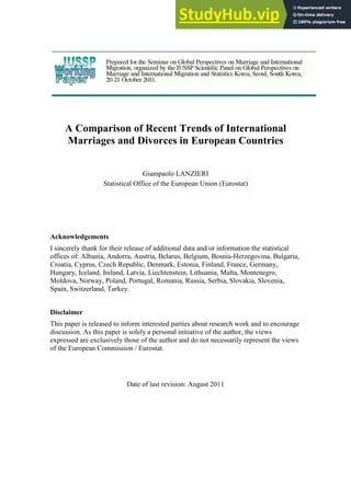
  • 28. 27 Figure 3: geographical patterns of international marriages and divorces (average 2005-09, expressed in per thousand persons for crude rates) Note: average over a shorter period for EL, LU, NL, PL, SI, SE. Apart Cyprus and Malta, and to a minor extent Liechtenstein and Luxembourg, the trends of international marriages and divorces are shaped by the corresponding trends of their mixed component, being the time series of foreign events usually more stable over time and on much lower levels. The Figure 4 shows the trends of crude rates of international events in the European countries grouped by region. Focussing first on international marriages (left side) and moving from top to bottom in Figure 4, in the Balkans the levels of the crude rates in Bosnia-Herzegovina and Croatia are very
  • 29. 28 similar; Slovenia has almost the double of their levels in the latest years, and Montenegro shows an increase following its independence from Serbia. The Baltic countries show a clear process of convergence. In Eastern Europe, there is a persistent degree of variability across countries, all of them on relatively low levels though. Romania and Bulgaria appears to be particularly volatile, Belarus shows a constant increase of the crude rate, and all the others have quite stable trends. The North- European countries all record in the latest years an increase of the rates, Denmark, Finland and Iceland moving together between Norway on the top and Sweden on the bottom. In Southern Europe, Cyprus shows a remarkable increase in 15 years, nothing comparable to any other European country; on a smaller scale, also Malta registers a significant step up in 2001-2003 of its crude rate, which remains almost stable afterwards. These two countries mask the trends of Greece, Italy, Portugal and Spain, which are all moving together, with a slight, constant increase after 2000. This characteristic of "moving together" in terms of crude rates can be traced also in several Western European countries: Austria, Belgium, France, Germany, the Netherlands, all of them mostly stable just below a level of one international marriage each thousand persons. Luxembourg and Switzerland also move together, but on higher levels, and Liechtenstein has partially converged to these latter countries, with variability distinctive of very small countries. The crude rates of international divorces (right side panels of Figure 4) have almost the same trends, but on much lower levels. However, some countries occasionally show odd values (Bulgaria, Switzerland), Denmark registers a sudden contraction between 2005 and 2007, and others have a different trend: in Montenegro international divorces fall down from the independence of the country, in Czech Republic they are instead constantly increasing. It could be argued that the observed levels of crude rates of international marriages and divorces may be simply following more general trends of decline or increase of marriages/divorces in the populations. On this latter aspect, Kalmijn (2007) provides already a cross-country comparison for Europe over the period 1990-2000, looking at the influence of various factors such as gender roles, religion, education and economic status, the former two being the most influential. In the Figure 5 are reported the proportion of international events on the total number of marriages (left panels) and divorces (right panels). Among Balkan countries, only
  • 30. 29 Montenegro has noticeably increased its quota of international marriages. Looking at the Baltic region, both in Estonia and Latvia international marriages loose a quota of several percentage points in the last decade, while in Lithuania the process is opposite, converging to the former two countries. In Eastern Europe, except Belarus, Bulgaria and Romania, the relative importance of international marriages remains almost stable, and for all of them on levels much lower than in the Baltic region. Among Northern- European countries, Iceland is the one with the highest increase of the quota of international marriages, from about 10% in the beginning of the Nineties to 23% 15 years later. Southern-European countries have all increased their share of international marriages from the end of the Nineties. In Western Europe, it is Switzerland to present the larger change over two decades, during which the share of international marriages has passed from above 30% to almost 50%. In other two countries of small size, Liechtenstein and Luxembourg, international marriages are regularly the majority. As for the quota of international divorces on the total number of these events, the right panels of Figure 5, there is a variety of cases: countries whose proportion of international divorces is increasing (e.g., Czech Republic), others in which is declining (e.g. Denmark), others again in which the quota is almost stable, or it is such in the latest period. Some additional explanations may be given about a few further countries' peculiarities which are visible in the Figure 4 and Figure 5. In Austria, the rate of international marriages has been oscillating around a level of one event every 1000 persons apart a peak registered in the years around 2004, when almost one out of three marriages was international. The decline which has followed afterwards is apparently in contradiction with the increasing stock of foreigners over the same years. In particular, the restriction to the single Austrian citizenship was not a problem for the Turks, one of the biggest community in the country, as Turkey was since 1995 – year of the accession of Austria to the EU- releasing a special card ensuring almost the same rights to those ex-Turkish citizens whishing to acquire the Austrian citizenship (Çinar 2010). A possible explanation may be related the entry into force in 2006 of a more restrictive policy on naturalisations (OECD 2010:190), which made the acquisition of citizenship to fall from almost 45 thousand in 2003 to 8 thousand in 2009 (Sartori 2009). Among the stricter requirements of the Austrian Federal Law amending the Nationality Law there is
  • 31. 30 a longer period of residence of the foreign spouse (5 years of uninterrupted residence in Austria) and of the marriage itself (six years) for his/her naturalisation through marriage. In fact, before 2005, a foreign spouse to Austrian citizen could apply for naturalisation even after three years and it can be noted that the number of international (mainly mixed) divorces has been increasing since 2003-2004, with a peak in 2007. Something alike may have occurred in Belgium, where after an almost constant proportion of 15% of international marriages, from 1997 there is a rapid increase up to 25% in 2004, year in which a decline starts. This turn down may be linked to the adoption of a more restrictive law on marriage: to the usual preventive approach against the marriages of convenience, the Belgian authorities have added in 2006 punitive measures to further curb this phenomenon, including the imprisonment (Foblets and Vanheule 2006). From that year, also the international divorces have re-started their rise, stopping again two years later. Data on Bulgaria and Romania reveal peculiar changes which may be related to the accession to the EU. The drop recorded in Switzerland in 2000 is due to the entry into force of a new Swiss law on divorce, which halved the number of events. The main change was meant to easier the procedure with the new profile of mutual agreement on the end of marriage, despite the introduction of non-fault grounds for divorce usually causes an increase of the cases (González and Viitanen 2006), in practice lawyers had difficulties to draw up such mutual acceptance. In lack of mutual consensus, the divorcing spouses have to go through a four-year separation period, which explains the time period, observed in the Figure 4, necessary to recover to the levels of crude rates pre-2000. Cyprus is the only country where the trends of the international marriages (but to a much less extent for divorces) are shaped by the (remarkable increase of the) foreign marriages and not by the mixed ones. Although the number of foreigners in the country has almost doubled since the accession of Cyprus to EU, the reason may be searched in the national wedding industry, which promotes the celebration of marriages between non-resident foreigners. This may also be the cause of the increasing number of foreign divorces which, although still fewer than the mixed divorces, have been increasing relentlessly in the past decade.
  • 32. 31 Figure 4: crude rates of international marriages and divorces in European regions 0.0 0.2 0.4 0.6 0.8 1.0 1.2 1.4 1.6 1.8 1990 1991 1992 1993 1994 1995 1996 1997 1998 1999 2000 2001 2002 2003 2004 2005 2006 2007 2008 2009 2010 BH HR ME SI region Balkan type event Marriages Crude Rates of International Events year country 0.0 0.1 0.2 0.3 0.4 0.5 0.6 0.7 1990 1991 1992 1993 1994 1995 1996 1997 1998 1999 2000 2001 2002 2003 2004 2005 2006 2007 2008 2009 2010 BH HR ME SI region Balkan type event Divorces Crude Rates of International Events year country 0.0 0.5 1.0 1.5 2.0 2.5 3.0 3.5 1990 1991 1992 1993 1994 1995 1996 1997 1998 1999 2000 2001 2002 2003 2004 2005 2006 2007 2008 2009 2010 EE LV LT region Baltic type event Marriages Crude Rates of International Events year country 0.0 0.5 1.0 1.5 2.0 2.5 3.0 3.5 4.0 1990 1991 1992 1993 1994 1995 1996 1997 1998 1999 2000 2001 2002 2003 2004 2005 2006 2007 2008 2009 2010 EE LV LT region Baltic type event Divorces Crude Rates of International Events year country 0.0 0.1 0.2 0.3 0.4 0.5 0.6 0.7 0.8 1990 1991 1992 1993 1994 1995 1996 1997 1998 1999 2000 2001 2002 2003 2004 2005 2006 2007 2008 2009 2010 BY BG CZ HU PL RO SK region Eastern type event Marriages Crude Rates of International Events year country 0.0 0.1 0.1 0.2 0.2 0.3 1990 1991 1992 1993 1994 1995 1996 1997 1998 1999 2000 2001 2002 2003 2004 2005 2006 2007 2008 2009 2010 BY BG CZ HU PL RO SK region Eastern type event Divorces Crude Rates of International Events year country 0.0 0.2 0.4 0.6 0.8 1.0 1.2 1.4 1.6 1.8 1990 1991 1992 1993 1994 1995 1996 1997 1998 1999 2000 2001 2002 2003 2004 2005 2006 2007 2008 2009 2010 DK FI IS NO SE region Northern type event Marriages Crude Rates of International Events year country 0.0 0.1 0.2 0.3 0.4 0.5 0.6 0.7 1990 1991 1992 1993 1994 1995 1996 1997 1998 1999 2000 2001 2002 2003 2004 2005 2006 2007 2008 2009 2010 DK FI IS NO SE region Northern type event Divorces Crude Rates of International Events year country 0.0 2.0 4.0 6.0 8.0 10.0 12.0 14.0 16.0 1990 1991 1992 1993 1994 1995 1996 1997 1998 1999 2000 2001 2002 2003 2004 2005 2006 2007 2008 2009 2010 CY EL IT MT PT ES region Southern type event Marriages Crude Rates of International Events year country 0.0 0.1 0.2 0.3 0.4 0.5 0.6 0.7 0.8 0.9 1.0 1990 1991 1992 1993 1994 1995 1996 1997 1998 1999 2000 2001 2002 2003 2004 2005 2006 2007 2008 2009 2010 CY EL IT MT PT ES region Southern type event Divorces Crude Rates of International Events year country 0.0 1.0 2.0 3.0 4.0 5.0 6.0 7.0 1990 1991 1992 1993 1994 1995 1996 1997 1998 1999 2000 2001 2002 2003 2004 2005 2006 2007 2008 2009 2010 AT BE FR DE LI LU NL CH region Western type event Marriages Crude Rates of International Events year country 0.0 0.2 0.4 0.6 0.8 1.0 1.2 1.4 1.6 1990 1991 1992 1993 1994 1995 1996 1997 1998 1999 2000 2001 2002 2003 2004 2005 2006 2007 2008 2009 2010 AT BE FR DE LI LU NL CH region Western type event Divorces Crude Rates of International Events year country
  • 33. 32 Figure 5: proportion of international marriages and divorces on the total number of events 0% 5% 10% 15% 20% 25% 30% 1990 1991 1992 1993 1994 1995 1996 1997 1998 1999 2000 2001 2002 2003 2004 2005 2006 2007 2008 2009 2010 BH HR ME SI region Balkan type event Marriages Proportion of international events year country 0% 10% 20% 30% 40% 50% 60% 70% 80% 1990 1991 1992 1993 1994 1995 1996 1997 1998 1999 2000 2001 2002 2003 2004 2005 2006 2007 2008 2009 2010 BH HR ME SI region Balkan type event Divorces Proportion of international events year country 0% 10% 20% 30% 40% 50% 60% 70% 1990 1991 1992 1993 1994 1995 1996 1997 1998 1999 2000 2001 2002 2003 2004 2005 2006 2007 2008 2009 2010 EE LV LT region Baltic type event Marriages Proportion of international events year country 0% 10% 20% 30% 40% 50% 60% 70% 80% 1990 1991 1992 1993 1994 1995 1996 1997 1998 1999 2000 2001 2002 2003 2004 2005 2006 2007 2008 2009 2010 EE LV LT region Baltic type event Divorces Proportion of international events year country 0% 2% 4% 6% 8% 10% 12% 14% 16% 1990 1991 1992 1993 1994 1995 1996 1997 1998 1999 2000 2001 2002 2003 2004 2005 2006 2007 2008 2009 2010 BY BG CZ HU PL RO SK region Eastern type event Marriages Proportion of international events year country 0% 1% 2% 3% 4% 5% 6% 7% 8% 1990 1991 1992 1993 1994 1995 1996 1997 1998 1999 2000 2001 2002 2003 2004 2005 2006 2007 2008 2009 2010 BY BG CZ HU PL RO SK region Eastern type event Divorces Proportion of international events year country 0% 5% 10% 15% 20% 25% 30% 35% 1990 1991 1992 1993 1994 1995 1996 1997 1998 1999 2000 2001 2002 2003 2004 2005 2006 2007 2008 2009 2010 DK FI IS NO SE region Northern type event Marriages Proportion of international events year country 0% 5% 10% 15% 20% 25% 30% 1990 1991 1992 1993 1994 1995 1996 1997 1998 1999 2000 2001 2002 2003 2004 2005 2006 2007 2008 2009 2010 DK FI IS NO SE region Northern type event Divorces Proportion of international events year country 0% 10% 20% 30% 40% 50% 60% 70% 80% 90% 1990 1991 1992 1993 1994 1995 1996 1997 1998 1999 2000 2001 2002 2003 2004 2005 2006 2007 2008 2009 2010 CY EL IT MT PT ES region Southern type event Marriages Proportion of international events year country 0% 5% 10% 15% 20% 25% 30% 35% 40% 45% 1990 1991 1992 1993 1994 1995 1996 1997 1998 1999 2000 2001 2002 2003 2004 2005 2006 2007 2008 2009 2010 CY EL IT MT PT ES region Southern type event Divorces Proportion of international events year country 0% 10% 20% 30% 40% 50% 60% 70% 80% 90% 1990 1991 1992 1993 1994 1995 1996 1997 1998 1999 2000 2001 2002 2003 2004 2005 2006 2007 2008 2009 2010 AT BE FR DE LI LU NL CH region Western type event Marriages Proportion of international events year country 0% 10% 20% 30% 40% 50% 60% 1990 1991 1992 1993 1994 1995 1996 1997 1998 1999 2000 2001 2002 2003 2004 2005 2006 2007 2008 2009 2010 AT BE FR DE LI LU NL CH region Western type event Divorces Proportion of international events year country
  • 34. 33 The level of aggregation of the data does not allow analysing in depth the reasons of cross-country and/or temporal variations of the proportion of international marriages/divorces. However, a factor which enters certainly in the picture is the presence of foreigners. The European countries present a large variety of migration experiences: some of them are historically immigration countries; others have rapidly changed from sending to receiving countries, others again are still basically emigration countries. In those two decades, a few countries had also implemented regularisations policies which made suddenly appearing in the statistics a large stock of illegal migrants. However, the sudden presence of a large number of foreigners may have a different influence on the international marriages than a smaller but older (in terms of residence in the country) stock of foreigners, due to the different time window of exposure to the risk of marriage. To incorporate this latter element, I consider the average quota of person-years of exposure of the foreigners over 6 years, from 2004 to 2009. In 2004 there has been the accession of ten countries to the European Union, which may have had an impact on the migratory flows, and therefore I have chosen to exclude the years before. To try minimising the influence of irregular years, I consider the average from 2007 to 2009 of the proportion of international marriages on the total number of events. Those countries for which data are missing are anyway included, the average being over the available years. The left panel of Figure 6 shows the high correlation between the two variables together with the regression line, whose intercept is not set to zero to allow for measurement errors. The value for Cyprus, on the top left, is an outlier due to the high quota of marriages celebrated by non-resident in that country: removing it makes the explicatory capacity of the quota of foreigners to increase from 61% to 77%, as shown in the right panel. Figure 6: scatter plot of the average proportion of international marriages 2007-09 and the average quota of foreigners 2004-09, with (left panel) and without (right panel) Cyprus y = 1.4823x + 0.1033 R2 = 0.6059 0% 10% 20% 30% 40% 50% 60% 70% 80% 0% 5% 10% 15% 20% 25% 30% 35% 40% 45% Foreigners International marriages CY y = 1.4096x + 0.0929 R2 = 0.7674 0% 10% 20% 30% 40% 50% 60% 70% 80% 0% 5% 10% 15% 20% 25% 30% 35% 40% 45% Foreigners International marriages
  • 35. 34 A further useful disaggregation would be the split of the foreigners' group in EU/non- EU citizenships, which would help to assess values and cultural differences. For divorces, the obvious dependence from the presence of foreigners is confirmed, as well as that from the proportion of international marriages. In one of the earlier studies dealing with the relation between divorces and migration, Thomas (1939) concludes that divorce is typical of urban culture, which is assimilated more slowly from migrants, who therefore show a more stable marital status. In her study, based on Swedish data, the focus was mostly on internal migrants; however, an exception was already noticed for migrants from distant communities in rural areas as for the proportion divorced. Recent research (Kalmijn et al. 2005) has shown that there is a higher risk of divorce for mixed nationality couples, even more than the highest level of divorce in the two homogamous groups. Zhang and Van Hook (2009) find that marital dissolution is indeed associated with ethnicity or race, but there is no evidence that interracial marriages are associated with higher risk of divorce, and controlling for citizenship did not alter the results. Taking into account the size of the groups, in general across Europe foreigners have (much) higher rates of marriage than nationals, and slightly more for divorce. The Table 5 reports the difference between the rates (29) and (34) for nationals and foreigners. Only a few countries (Germany, Greece, Latvia and Spain) have marriage/marrying persons' rates for nationals on comparable levels of those for foreigners; for all the others, the differences are remarkable, and sometimes extreme, even though in these latter cases high caution should be applied. Table 5: average events and persons rates 2006-07 for nationals and foreigners Extended group-specific crude rates (x1000) Group-specific persons rates (x1000) Marriages Divorces Marrying Divorcing Nat For Diff Nat For Diff Nat For Diff Nat For Diff AT 4.2 6.5 -2.3 2.4 3.4 -1.0 8.3 13.0 -4.7 4.7 6.8 -2.1 BE 4.0 6.8 -2.8 2.7 3.5 -0.7 8.0 13.6 -5.6 5.5 6.9 -1.5 BG 3.9 65.6 -61.7 2.0 18.3 -16.3 7.7 131.1 -123.4 4.0 36.7 -32.7 CY 6.0 94.8 -88.8 1.8 4.8 -2.9 12.1 189.7 -177.6 3.7 9.5 -5.9 CZ 5.3 8.2 -3.0 3.0 3.5 -0.5 10.5 16.4 -5.9 6.0 7.0 -1.0 DK 6.3 13.3 -7.0 2.5 5.5 -3.0 12.7 26.6 -14.0 4.9 11.0 -6.1 EE 4.9 6.5 -1.6 2.7 3.5 -0.8 9.8 12.9 -3.1 5.4 7.0 -1.7 FI 5.4 15.2 -9.9 2.4 7.2 -4.8 10.7 30.5 -19.8 4.8 14.3 -9.6 FR 4.3 4.9 -0.7 8.5 9.9 -1.3 DE 4.5 4.1 0.4 2.2 3.0 -0.7 9.1 8.3 0.8 4.5 5.9 -1.5 EL 5.4 5.1 0.2
  • 36. 35 HU 4.2 6.8 -2.6 2.5 1.5 1.0 8.4 13.5 -5.1 5.0 3.0 2.0 IS 5.5 10.1 -4.6 1.7 2.1 -0.5 11.0 20.2 -9.2 3.3 4.3 -0.9 IT 4.0 7.6 -3.5 0.9 0.2 0.6 8.0 15.1 -7.1 LV 6.7 6.1 0.6 13.4 12.3 1.2 LI 3.9 6.3 -2.4 7.8 12.6 -4.8 LU 4.0 4.3 -0.4 2.6 2.2 0.4 LT 6.2 34.6 -28.4 3.3 9.6 -6.3 12.4 69.2 -56.7 6.5 19.1 -12.6 MT 4.4 55.5 -51.1 8.9 111.0 -102.1 NL 4.2 9.6 -5.3 1.8 4.8 -3.0 NO 4.5 16.8 -12.4 9.0 33.7 -24.7 PL 6.2 36.4 -30.2 12.4 72.8 -60.4 PT 4.3 8.2 -3.9 2.3 1.3 1.0 8.6 16.4 -7.8 4.6 2.7 1.9 RO 7.6 131.1 -123.4 1.6 7.1 -5.5 15.3 262.1 -246.8 3.2 14.1 -10.9 SK 4.6 56.5 -51.9 2.3 3.5 -1.2 9.3 113.0 -103.7 4.6 7.1 -2.5 SI 2.9 11.2 -8.2 1.2 2.4 -1.2 5.9 22.3 -16.4 2.4 4.9 -2.5 ES 4.6 4.6 0.0 2.9 2.1 0.8 9.3 9.3 0.0 5.8 4.1 1.7 SE 4.8 11.6 -6.8 2.0 6.9 -4.9 CH 4.7 7.9 -3.2 2.4 4.1 -1.7 9.3 15.7 -6.4 4.7 8.2 -3.4 Avg 4.9 22.6 -17.7 2.2 4.6 -2.3 9.9 50.0 -40.2 4.6 9.6 -5.0 In the future, it may be expected an increase of international marriages and, consequently, of the international divorces. Due to the progressive ageing of the European populations (Lanzieri, 2011), the immigration flows are assumed to continue and to influence the future population structures, giving origin to more diverse societies especially at younger ages (Lanzieri 2010). Therefore, while the number of national marriages may be shrinking in the future simply because the number of nationals in marriageable age may be declining, as the immigrants are usually younger than the host populations (Oblak Flander 2011), marriages involving at least one foreigner are likely to increase instead, if not in numbers at least in proportion. The impact of migrants' descents on international marriages is not easy to disentangle, because it depends as well on the legislative setting in the country about citizenship. As they are likely to be more open to unions with person of the host country, more exogamous marriages may occur, recorded as mixed or national marriage depending on the citizenship of the second generation of migrants. If instead the continuous inflow of immigrants reduces the push factors to exogamy of these offspring, the increasing endogamous marriage may appear as mixed or foreign event, again depending on the citizenship laws of the country. Offspring of mixed unions are instead likely to have the citizenship of the host country and to be as well more open to exogamous marriages. Therefore, their contribution to international marriages, and in particular on the mixed ones, is expected to be positive.
  • 37. 36 In general, whether the marriages occur between nationals and foreigners, or between nationals and between foreigners, is also a matter of integration/assimilation in the host country. To dig further into this subject, it is necessary to break down the international marriages in its two components. In fact, mixed marriages and foreign marriages are expression respectively of exogamy and endogamy. Strictly speaking, foreign marriages could be considered measures of both endogamy and exogamy, if one takes into account that foreigners are actually a rather heterogeneous group, and events may well refer to persons of different citizenship, although both foreigners. 6. Exogamy and endogamy in European countries Using the measures selected in the Table 3, the available values covering the period 1990-2010 are reported in the Table 9 as averages of 5-year age groups for 33 European countries. This is actually a quite comprehensive test of the performances of the selected indicators, because in that set are included countries of both small and big population size, countries with different union formation patterns (little or widespread cohabitation/registered partnership), old and new immigration – or still emigration - countries, some having experienced a sudden increase of the immigration flows. Further, there are countries where the number of events under consideration is very small, or even there are none, and others where they are much more common, possibly unbalanced between sexes. Last but not least, the different data availability and quality are further elements of test of these measures. Due to its data requirements, values for 2 Z are the less available among the selected indicators, and always missing for 2010. In particular, it was not possible to compute 2 Z for Belarus, Bosnia-Herzegovina and Croatia due to the missing information on population by citizenship; necessary data for 2 Z as well as for other indicators were not available for Greece, Luxembourg, Netherlands and Sweden, due to the missing breakdown of marriages by citizenship of each spouse. With a few exceptions, the indicators point out a state of endogamy in Europe, although with different degrees depending on the chosen measure. A description of the trends country by country would be too lengthy and I will then only highlight a few issues of similarity/dissimilarity across countries and the behaviour of the selected indicators. For
  • 38. 37 sake of simplicity, I consider values of the indicators between 0 and 0.25 (with plus or minus sign, depending if respectively on the exogamy or endogamy side) as almost not significant and therefore indicative of indifference, those between 0.25 and 0.50 as indicative of a weak intensity of exogamy/endogamy, moderate intensity for values between 0.50 and 0.75, and finally strong exogamy/endogamy for values between 0.75 and 1, this latter value corresponding to the maximum possible. As expected from the simulations reported in Figure 2, 2 mix e tends to assume values higher than the other indexes, falling mostly in the bandwidth of indifference. On the contrary, the other basic measure, 2 mix m , takes almost always values indicative of moderate/strong endogamy, sometimes in contradiction with all the other indicators (e.g., see Bulgaria, or Czech Republic). Liechtenstein is the only country where this indicator moves within the area of indifference. Trends of 2 mix m are quite stable over time, although the indicator does show changes (like in Austria, Portugal or Spain). Being the less demanding measure in terms of data requirement, 2 mix m and 2 mix e are the only indicators which can be computed for all European countries. The average proportion of intermarrying persons, 2 mix s , takes values very close to the index 2 H . The message from these two indicators is almost identical: moderate endogamy for Cyprus and Malta, weak endogamy for few countries (Denmark, Estonia, Finland and Italy), a bunch of others (Austria, Belgium, France, Iceland, Latvia, Spain and Switzerland) between weak endogamy and indifference, indifference in all the rest. An exception is Croatia, where these two measures move apart each other, although this seems to be a statistical effect of the cross-products. As expected, 2 std H returns a higher intensity of endogamy, although in general it takes values close to 2 H . Major differences between these two indicators are again in Croatia, as well as in Finland, Italy and Montenegro, and to a less extent in few other countries. According to 2 std H , there are a few more countries than with the previous two indicators ( 2 H and 2 mix s ) with moderate endogamy, and others shift from indifference to weak endogamy. Thus, apart the four countries listed above, there are no major changes in meaning by using one or the other version of the indicator H, although the countries' ranking may be slightly more sensitive to the choice.
  • 39. 38 Like 2 H and 2 std H , 2 Q becomes undetermined with multiple zero frequencies. Further, in order to avoid the statistical artefact of unitary values in presence of a zero frequency, as it occurs for Romania, Slovakia and Slovenia for foreign marriages in selected years, I removed these cases from the computations. The real peculiarity of this indicator is its volatility: in general, either 2 Q takes the highest/lowest values among the set of indicators, or it changes rapidly, even moving from endogamy to exogamy (like for Belarus and Lithuania) or vice versa (like for Czech Republic) in a few years. The matter is its sensitivity to changes in the cross-products of the Table 1, to a higher extent than 2 H and 2 std H . That such variability could reflect a real change of the propensity to marry with persons of a specific group, or at least to that extent, should be matter of further thoughts. The picture that would emerge about Europe using this indicator would be of countries with higher intensities of endogamy or exogamy, the majority of them showing moderate or strong propensities; fluctuations as well would be wider than for other indicators. On the whole, the transformation 2 V of the Gray's index of marital distance behaves much more smoothly, almost alike the set of three indicators 2 mix s , 2 H and 2 std H , although in some countries differences may be remarkable. Further, 2 V may also diverge from that set of indicators (Bulgaria, Italy), or converge to (Latvia, Portugal), or cross them (Belarus, Czech Republic, Lithuania, Spain), though, by and large, the message that can be got from the four indicators all together is almost consistent. An issue for 2 V is that, when there are no foreign marriages, it takes values close to 0.5, regardless of the value assumed the year before or after, and this may turn out in odd trends, as in the case of Romania, Slovakia and Slovenia. The indicator 2 Z is the only that may signals exogamy, or a tendency to, when all the other measures indicate endogamy. The additional information about the population exposed to the risk makes indeed the difference for some countries, and anyway contributes to shape differently the trends of this indicator, which generally (but not always: see for instance Cyprus) takes higher values then the others. Unfortunately, the available time series are shorter and the territorial coverage smaller than for any other indicator; further, by definition, 2 Z is also sensitive to changes in the population at risk.
  • 40. 39 According to this indicator, the situation in Europe in the second half of the last decade sees Cyprus to manifest a strong endogamy, followed by Malta with a moderate propensity to marry within the own group (see Figure 7). There is then a bunch of countries (Italy, Spain, Estonia and Latvia) on the border within weak endogamy and indifference, followed by several others where the citizenship does not really play a role in the choice of the partner, most of them located in Central Europe. Slovenia, Poland and Lithuania manifest moderate exogamy, and for three Eastern Europe countries (Bulgaria, Romania and Slovakia) there is evidence of strong exogamy. Figure 7: average of the values 2005-09 of Z2 by country, sorted by ascending order (countries marked by star have the average computed on a shorter period) -1.00 -0.75 -0.50 -0.25 0.00 0.25 0.50 0.75 1.00 CY MT IT ES EE LV DE DK FR BE AT FI IS CH PT LI* HU NO CZ SI* PL* LT SK BG* RO* However, attention should be paid to the statistical effects and to the quality of the data. Values for Cyprus and probably also for Malta are affected by the inclusion of marriages of non-residents in the statistics, and therefore one may expect the value for these two countries to be biased downward. The other peculiar set of countries is on the right side of the Figure 7. A possible explanation is that those countries are now the gate to European Union for neighbouring countries. For instance, in Slovenia there is a relatively high presence of persons from ex-Yugoslavian states (Bosnia-Herzegovina, Macedonia, etc.), in Poland and Slovakia of Ukrainians (Vasileva, 2011). For Poland,
  • 41. 40 Górny and Kępińska (2004) highlights the importance of temporary labour migration from Ukraine to Poland for the Ukrainian-Polish mixed marriages in Poland, not excluding the occurrence of bogus marriages with Polish citizens for the sake of an easy acquisition of a Permanent Residence Permit. As such temporary movements are not included in the usual statistics on migrants, where the rule of usual residence for at least 12 months is used, and they may have outnumbered the settled migrants, the population of reference for Z2 may be biased and consequently the values of Z2 less reliable for Poland. Bulgaria, Lithuania, Poland, Romania and Slovakia have the smallest quotas of foreigners, and very few foreign marriages, which may explain the higher values of Z2 , but also issues of data quality and consistency may play a role. The trends by region showed in the various panels of the Figure 8 highlight the similarities between countries: for instance, between Estonia and Latvia, or Hungary and Czech Republic, between Bulgaria, Romania and Slovakia, Spain and Italy, or again between all Northern European countries, and finally between all Western European countries. It is interesting to note how, once controlling for sex and group composition of the population, small countries like Liechtenstein or Luxembourg cease to be extreme cases, as it would appear looking only at rates or proportion of international marriages. For the Balkan region, the unfortunate scarcity of information about the stock of migrants does not allow the computation of the index for most of its countries. Several studies (Botev 1994, Mrdjen 2000, Smits 2010) have addressed the issue of inter-ethnic marriages in the former Yugoslavia until the end of the Eighties. Their findings are difficult to compare with the current data, not only because they were based on analysis of the nationalities (corresponding to ethnic groups), which may not be completely "translated" in citizenships nowadays, but also because they refer to a social context rather different from the one after the wars in the Balkans (1991-95 and 1998-99 in different parts of the region).
  • 42. 41 Figure 8: trends of the indicator Z2 by European region -1.00 -0.75 -0.50 -0.25 0.00 0.25 0.50 0.75 1.00 1998 1999 2000 2001 2002 2003 2004 2005 2006 2007 2008 2009 BH HR ME SI region Balkan type event Marriages Indicator Z2 year country -1.00 -0.75 -0.50 -0.25 0.00 0.25 0.50 0.75 1.00 1998 1999 2000 2001 2002 2003 2004 2005 2006 2007 2008 2009 EE LT LV region Baltic type event Marriages Indicator Z2 year country -1.00 -0.75 -0.50 -0.25 0.00 0.25 0.50 0.75 1.00 1998 1999 2000 2001 2002 2003 2004 2005 2006 2007 2008 2009 BG BY CZ HU PL RO SK region Eastern type event Marriages Indicator Z2 year country -1.00 -0.75 -0.50 -0.25 0.00 0.25 0.50 0.75 1.00 1998 1999 2000 2001 2002 2003 2004 2005 2006 2007 2008 2009 DK FI IS NO SE region Northern type event Marriages Indicator Z2 year country -1.00 -0.75 -0.50 -0.25 0.00 0.25 0.50 0.75 1.00 1998 1999 2000 2001 2002 2003 2004 2005 2006 2007 2008 2009 CY EL ES IT MT PT region Southern type event Marriages Indicator Z2 year country -1.00 -0.75 -0.50 -0.25 0.00 0.25 0.50 0.75 1.00 1998 1999 2000 2001 2002 2003 2004 2005 2006 2007 2008 2009 AT BE CH DE FR LI LU NL region Western type event Marriages Indicator Z2 year country Also the Baltic region went through a period of social change, following the independence from the USSR in 1991. In Latvia and Estonia, countries which show a remarkable similarity in intermarriages trends (see Figure 4, Figure 5 and Figure 8), there has been a renewed consciousness of the national identity, and the ethnic Russian shifted to a position of minority group (Monden and Smits 2005, van Ham and Tammaru 2011). The citizenship laws adopted in these countries were particularly attentive to preserve the recent independence from foreign influences, approach that together with the contemporary collapse of the Soviet Union left without citizenship a large number of residents of different ethnicity, mostly Russians, later recognised as "non-citizen" or "with undefined citizenship" (Krūma 2010, Järve and Poleshchuk 2010). Analysing the period 1970-2003, Monden and Smits (2005) find an increase of intermarriages between ethnics Latvians and Russians, measured by the reduction of the
  • 43. 42 odds ratio after 1990, which they explain by changes in the migration patterns: the least integrated Russians (like those serving in the army) had emigrated from Latvia, and those remained were more keen to integration. Considering that many ethnic Russians may have turned to be non-citizens and thus foreigners in the current study, and that they are the prevalent minority group in Latvia (Vasileva 2011), the results from Monden and Smits (2005) can be partially compared with the observed level of Z2 . While they base themselves on the reduction of the odds ratio (which in fact continues in the years after 2003) to support the hypothesis of the reduction of the social distances, taking into account the reduced intra-marriage opportunities for foreigners (i.e., ethnic Russians), estimated to reduce by more than 40% from 1998 to 2009, according to the index Z2 the level of endogamy remains almost stable in the latest years, implying little – if any - reduction of the social distances. Unfortunately, there is almost no overlapping between the time period examined by Monden and Smits (2005) and the one available here for Latvia for Z2 , but as the odds ratio continue to decrease after 2003 (although slowing down), their conclusions may be supposed to apply even further. Taking into account that Monden and Smits clarify that the change in preferences concerns only the Russians and not the Latvians, the findings may still be matched looking at the disaggregation by citizenship group. As for Estonia, van Ham and Tammaru (2011) highlight the characteristics of occupational, educational and spatial segregation of the Estonian society, and the higher likelihood of second- and third-generation immigrant to enter inter-ethnic marriages, whereas the index Z2 indicates a very slow change from weak endogamy to indifference in the latest year for mixed citizenship marriages. Lithuania has a quota of foreigners much lower than Latvia and Estonia, which may explain the difference between these Baltic countries. 7. Analysis by gender and citizenship group The three indicators 2 mix s , 2 V and 2 Z allow a disaggregation by gender and citizenship group, which can be particularly helpful to gain further insights in the endogamy/exogamy analysis. In fact, each of them is the outcome of an operation done on sex- and group-specific components. For sake of simplicity, such basic components can be analysed without transforming them to range into the interval [-1,+1].