Download as PDF, PPTX


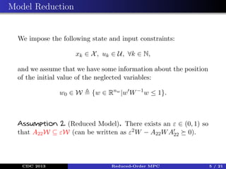
![The MPC formulation
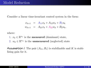
Let us introduce the sets
Z
X
ˆ(∞)
SK
V
U
ˆ(∞)
K SK ,
Along the prediction horizon N we impose the constraints:
zk ∈ Z, ∀k ∈ N[1,N −1]
vk ∈ V, ∀k ∈ N[0,N −1]
and the terminal constraint
zN ∈ Zf .
CDC 2013
Reduced-Order MPC
9 / 21](https://image.slidesharecdn.com/sopberbem13cdc-131211183105-phpapp02/85/Model-Predictive-Control-based-on-Reduced-Order-Models-9-320.jpg)
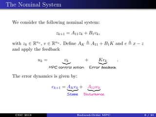
![The MPC optimization problem is:
PN (z) : VN (z) = min VN (z, v),
v∈V(z)
where the cost function is given by:
N −1
VN (z, v)
zN P zN +
zk QzK + vk Rvk ,
k=0
and V(z) is the following multi-valued mapping:
z0 =z,
z =A11 zk +B1 vk , ∀k∈N[1,N −1] ,
V(z)
v k+1
zk ∈ Z, ∀k∈N[1,N −1] ,
vk ∈ V, ∀k∈N[0,N −1] , zN ∈ Zf
CDC 2013
Reduced-Order MPC
.
10 / 21](https://image.slidesharecdn.com/sopberbem13cdc-131211183105-phpapp02/85/Model-Predictive-Control-based-on-Reduced-Order-Models-10-320.jpg)
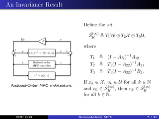
![Exponential Robust Stability
Let κN be the MPC control action and
κN (z, x) = K(x − z) + κN (z).
˜
ˆ(∞)
The set SK × {0} is exponentially stable for the system
xk+1 = A11 xk + B1 (˜ N (zk , xk )) + A12 wk
κ
zk+1 = A11 zk + B1 κN (zk ),
(with state variable [ x ]) over the domain of attraction
z
(∞)
ˆ
(ZN ⊕ SK ) × ZN .
CDC 2013
Reduced-Order MPC
11 / 21](https://image.slidesharecdn.com/sopberbem13cdc-131211183105-phpapp02/85/Model-Predictive-Control-based-on-Reduced-Order-Models-11-320.jpg)

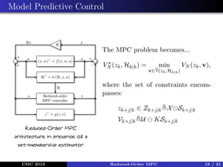
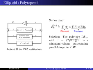
![Exponential Robust Stability
Stability Result:
Assume that Hk|k → H and let S
(I − AK )−1 H . The set
S × {0}
is exponentially stable for the dynamics of [ x ].
z
Reduced-Order MPC
architecture in presence of a
set-membership estimator.
CDC 2013
Reduced-Order MPC
17 / 21](https://image.slidesharecdn.com/sopberbem13cdc-131211183105-phpapp02/85/Model-Predictive-Control-based-on-Reduced-Order-Models-17-320.jpg)
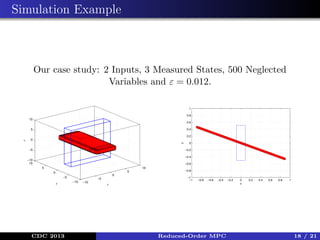
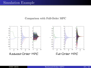
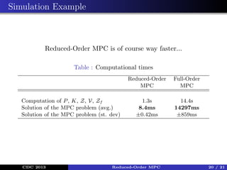


This document presents a method for model predictive control (MPC) using reduced-order models. Many physical systems are modeled using partial differential equations with thousands of states, making MPC computationally challenging. The method reduces the model order by treating some states as disturbances and estimating their bounds. An invariance result shows the error remains bounded. The MPC optimization problem is formulated subject to the reduced constraints. Simulation results show the reduced-order MPC matches full-order MPC performance while being significantly faster to compute.