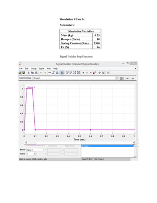
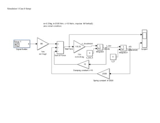
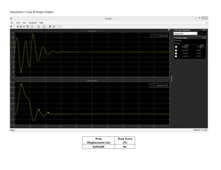
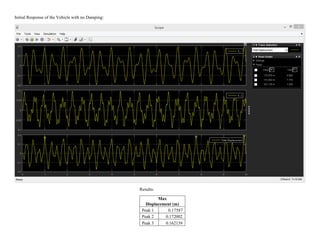
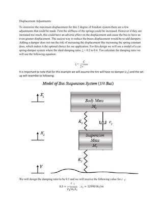
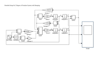
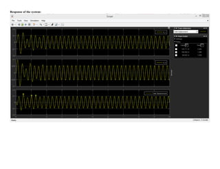
Final Simulation
Vibrations
Project Kevin O'Connor
April 16, 2016
Professor Ma
Simulation 1 Case A : Diagram of Setup:
Simulation Variables
Mass (kg) 0.25
Damper (Ns/m) 10
Spring Constant (N/m) 2500
F_o (N) 26
Tau (seconds) 0.001
Length of Step (seconds) 0.001
Equation of Motion: 𝑘𝑘
𝑚𝑚𝑥𝑥̈ + 𝑐𝑐𝑥𝑥̇ + 𝑘𝑘𝑥𝑥 = 𝐹𝐹(𝑡𝑡)
0.25𝑥𝑥̈ + 10𝑥𝑥̇ + 2500𝑥𝑥 = 28𝛿𝛿(0)
Simulation 1 Case A Setup:
Simulation 1 Case A Signal Builder:
Simulation 1 Case A Scope Output:
Peak
Displacement (m)
Peak Force
(N)
0.000845 26
Simulation 1 Case b:
Parameters:
Simulation Variables
Mass (kg) 0.25
Damper (Ns/m) 10
Spring Constant (N/m) 2500
Fo (N) 96
Signal Builder Step Function:
Simulation 1 Case b Setup:
Simulation 1 Case B Scope Output:
Peak
Displacement (m)
Peak Force
(N)
0.054189 96
Part C: MATLAB Code:
MATLAB Graph Output:
𝑠𝑠𝑠𝑠
Conclusion:
The MATLAB theoretical solution presented in the graph above uses the convolution integral taken with respect to tau to
solve the step function in part a. I have used MATLAB to solve the complex integral needed to integrate a damped step
function and then have plotted it. It should be noted that the blue wave form is the displacement of the system from time 0
< 𝑡𝑡 < 0.001 and the yellow wave form is the displacement of the system from time 𝑡𝑡 > 0.001. The theoretical
simulation using the convolution integral results in a maximum value of approximately 0.0175 meters and the Simulink
simulation results in a maximum value of 0.00845 meters. However it should be noted that when the time increment of
the simulation is decreased the accuracy of the simulation increases as well.
Simulation Part2:
Parameters:
Simulation Inputs
First Name Initial, K 11
Last Name Initial, O 15
Spring Constant,
k1 (N/m) 452000
Spring Constant,
k2 (N/m) 500000
Mass, m1 (kg) 1026
Mass, m2 (kg) 300
Amplitude, Y(m) 0.1
Period, L(m) 6
Velocity, v(kph) 80
Frequency, w(rad/s) 23.27106
Equation of Motion:
𝑚𝑚1 𝑥𝑥1̈ + 𝑘𝑘1(𝑥𝑥2 − 𝑥𝑥1) = 0
1028𝑥𝑥1̈ + 456000(𝑥𝑥2 − 𝑥𝑥1) = 0 𝑒𝑒𝑒𝑒: (1)
𝑚𝑚2 𝑥𝑥2̈ + 𝑘𝑘2(𝑥𝑥2 − 𝑦𝑦) − 𝑘𝑘1(𝑥𝑥2 − 𝑥𝑥1) = 0
300𝑥𝑥2̈ + 44000𝑥𝑥2 + 456000𝑥𝑥1 = 500000𝑦𝑦 𝑒𝑒𝑒𝑒: (2)
Simulink Setup for Part 1:
Initial Response of the Vehicle with no Damping:
Results:
Max
Displacement (m)
Peak 1 0.17587
Peak 2 0.172002
Peak 3 0.162139
Displacement Adjustments:
To minimize the maximum displacement for this 2 degree of freedom system there are a few
adjustments that could be made. First the stiffness of the springs could be increased. However if they are
increased too much, this could have an adverse effect on the displacement and cause the bus to have an
even greater displacement. The easiest way to reduce the buses displacement would be to add dampers.
Adding a damper does not run the risk of increasing the displacement like increasing the spring constant
does, which makes it the optimal choice for our application. For this design we will use a model of a car
spring-damper system where the ideal damping ratio, ζ = 0.2 to 0.4. Too calculate the damping ratio we
will use the following equation:
ζ =
𝐶𝐶
𝑚𝑚
It is important to note that for this example we will assume the tire will have no damper (𝑐𝑐2) and the set
up will resemble to following:
0.3 =
2�𝑚𝑚1 𝑘𝑘1
We will design the damping ratio to be 0.3 and we will receive the following value for 𝑐𝑐 1:
𝑐𝑐 1
, 𝑐𝑐1 = 12990 𝑁𝑁𝑁𝑁/𝑚𝑚
Parameters:
Simulation Inputs
First Name Initial, K 11
Last Name Initial, O 15
Spring Constant,
k1 (N/m) 452000
Spring Constant,
k2 (N/m) 500000
Damper, c1 (Ns/m) 12990
Mass, m1 (kg) 1028
Mass, m2 (kg) 300
Amplitude, Y(m) 0.1
Period, L(m) 6
Velocity, v(kph) 80
Frequency, w(rad/s) 23.27106
Equations of Motion:
𝑚𝑚1 𝑥𝑥1̈ + 𝑐𝑐1(𝑥𝑥̇2 − 𝑥𝑥̇1) + 𝑘𝑘1(𝑥𝑥2 − 𝑥𝑥1) = 0
1028𝑥𝑥1̈ + 1300(𝑥𝑥̇2 − 𝑥𝑥̇1) + 456000(𝑥𝑥2 − 𝑥𝑥1) = 0 𝑒𝑒𝑒𝑒: (1)
𝑚𝑚2 𝑥𝑥2̈ − 𝑐𝑐1(𝑥𝑥2̇ − 𝑥𝑥̇1) + 𝑘𝑘2(𝑥𝑥2 − 𝑦𝑦) − 𝑘𝑘1(𝑥𝑥2 − 𝑥𝑥1) = 0
300𝑥𝑥2̈ − 1300(𝑥𝑥̇2 − 𝑥𝑥̇1) + 44000𝑥𝑥2 + 456000𝑥𝑥1 = 500000𝑦𝑦 𝑒𝑒𝑒𝑒: (2)
Simulink Setup for 2 Degree of Freedom System with Damping:
Response of the system:
Results:
When damping is added there is a significant decrease in the displacement of the bus, which can be seen
below in the table.
Before Damping
Displacement (m)
Damping Added
Displacement (m)
% Reduction in
Displacement (%)
Peak 1 0.17587 0.120211 30.36
Peak 2 0.172002 0.100011 40.75
Peak 3 0.162139 0.089022 37.69
When we compare the scope without damping to the one with damping there is also a significant change
in the shape of the “Total Displacement” plot. Without damping, the plot had many peaks, and the total
displacement never came close to the input displacement of 0.1 meters. When damping is added however
there is a peak in the “Total Displacement” initially but this is quickly compensated for by the damping
and within 2 seconds, the “Total Displacement” plot is only displacing the input displacement of 0.1
meters. This is the important take away from this simulation, that when dampers are added the car does
not continue to have peak displacements across the entire simulation, which is what was observed in the
initial simulation. The dampers are working to absorb the input of the road and rebound of the springs,
which is clearly evident in the shape of the scope plots.

OConnor_SimulationProject

  • 1.
    Final Simulation Vibrations Project KevinO'Connor April 16, 2016 Professor Ma
  • 2.
    Simulation 1 CaseA : Diagram of Setup: Simulation Variables Mass (kg) 0.25 Damper (Ns/m) 10 Spring Constant (N/m) 2500 F_o (N) 26 Tau (seconds) 0.001 Length of Step (seconds) 0.001 Equation of Motion: 𝑘𝑘 𝑚𝑚𝑥𝑥̈ + 𝑐𝑐𝑥𝑥̇ + 𝑘𝑘𝑥𝑥 = 𝐹𝐹(𝑡𝑡) 0.25𝑥𝑥̈ + 10𝑥𝑥̇ + 2500𝑥𝑥 = 28𝛿𝛿(0)
  • 3.
  • 4.
    Simulation 1 CaseA Signal Builder:
  • 5.
    Simulation 1 CaseA Scope Output: Peak Displacement (m) Peak Force (N) 0.000845 26
  • 6.
    Simulation 1 Caseb: Parameters: Simulation Variables Mass (kg) 0.25 Damper (Ns/m) 10 Spring Constant (N/m) 2500 Fo (N) 96 Signal Builder Step Function:
  • 7.
  • 8.
    Simulation 1 CaseB Scope Output: Peak Displacement (m) Peak Force (N) 0.054189 96
  • 9.
  • 10.
  • 11.
    𝑠𝑠𝑠𝑠 Conclusion: The MATLAB theoreticalsolution presented in the graph above uses the convolution integral taken with respect to tau to solve the step function in part a. I have used MATLAB to solve the complex integral needed to integrate a damped step function and then have plotted it. It should be noted that the blue wave form is the displacement of the system from time 0 < 𝑡𝑡 < 0.001 and the yellow wave form is the displacement of the system from time 𝑡𝑡 > 0.001. The theoretical simulation using the convolution integral results in a maximum value of approximately 0.0175 meters and the Simulink simulation results in a maximum value of 0.00845 meters. However it should be noted that when the time increment of the simulation is decreased the accuracy of the simulation increases as well.
  • 12.
    Simulation Part2: Parameters: Simulation Inputs FirstName Initial, K 11 Last Name Initial, O 15 Spring Constant, k1 (N/m) 452000 Spring Constant, k2 (N/m) 500000 Mass, m1 (kg) 1026 Mass, m2 (kg) 300 Amplitude, Y(m) 0.1 Period, L(m) 6 Velocity, v(kph) 80 Frequency, w(rad/s) 23.27106 Equation of Motion: 𝑚𝑚1 𝑥𝑥1̈ + 𝑘𝑘1(𝑥𝑥2 − 𝑥𝑥1) = 0 1028𝑥𝑥1̈ + 456000(𝑥𝑥2 − 𝑥𝑥1) = 0 𝑒𝑒𝑒𝑒: (1) 𝑚𝑚2 𝑥𝑥2̈ + 𝑘𝑘2(𝑥𝑥2 − 𝑦𝑦) − 𝑘𝑘1(𝑥𝑥2 − 𝑥𝑥1) = 0 300𝑥𝑥2̈ + 44000𝑥𝑥2 + 456000𝑥𝑥1 = 500000𝑦𝑦 𝑒𝑒𝑒𝑒: (2)
  • 13.
  • 14.
    Initial Response ofthe Vehicle with no Damping: Results: Max Displacement (m) Peak 1 0.17587 Peak 2 0.172002 Peak 3 0.162139
  • 15.
    Displacement Adjustments: To minimizethe maximum displacement for this 2 degree of freedom system there are a few adjustments that could be made. First the stiffness of the springs could be increased. However if they are increased too much, this could have an adverse effect on the displacement and cause the bus to have an even greater displacement. The easiest way to reduce the buses displacement would be to add dampers. Adding a damper does not run the risk of increasing the displacement like increasing the spring constant does, which makes it the optimal choice for our application. For this design we will use a model of a car spring-damper system where the ideal damping ratio, ζ = 0.2 to 0.4. Too calculate the damping ratio we will use the following equation: ζ = 𝐶𝐶 𝑚𝑚 It is important to note that for this example we will assume the tire will have no damper (𝑐𝑐2) and the set up will resemble to following: 0.3 = 2�𝑚𝑚1 𝑘𝑘1 We will design the damping ratio to be 0.3 and we will receive the following value for 𝑐𝑐 1: 𝑐𝑐 1 , 𝑐𝑐1 = 12990 𝑁𝑁𝑁𝑁/𝑚𝑚
  • 16.
    Parameters: Simulation Inputs First NameInitial, K 11 Last Name Initial, O 15 Spring Constant, k1 (N/m) 452000 Spring Constant, k2 (N/m) 500000 Damper, c1 (Ns/m) 12990 Mass, m1 (kg) 1028 Mass, m2 (kg) 300 Amplitude, Y(m) 0.1 Period, L(m) 6 Velocity, v(kph) 80 Frequency, w(rad/s) 23.27106 Equations of Motion: 𝑚𝑚1 𝑥𝑥1̈ + 𝑐𝑐1(𝑥𝑥̇2 − 𝑥𝑥̇1) + 𝑘𝑘1(𝑥𝑥2 − 𝑥𝑥1) = 0 1028𝑥𝑥1̈ + 1300(𝑥𝑥̇2 − 𝑥𝑥̇1) + 456000(𝑥𝑥2 − 𝑥𝑥1) = 0 𝑒𝑒𝑒𝑒: (1) 𝑚𝑚2 𝑥𝑥2̈ − 𝑐𝑐1(𝑥𝑥2̇ − 𝑥𝑥̇1) + 𝑘𝑘2(𝑥𝑥2 − 𝑦𝑦) − 𝑘𝑘1(𝑥𝑥2 − 𝑥𝑥1) = 0 300𝑥𝑥2̈ − 1300(𝑥𝑥̇2 − 𝑥𝑥̇1) + 44000𝑥𝑥2 + 456000𝑥𝑥1 = 500000𝑦𝑦 𝑒𝑒𝑒𝑒: (2)
  • 17.
    Simulink Setup for2 Degree of Freedom System with Damping:
  • 18.
  • 19.
    Results: When damping isadded there is a significant decrease in the displacement of the bus, which can be seen below in the table. Before Damping Displacement (m) Damping Added Displacement (m) % Reduction in Displacement (%) Peak 1 0.17587 0.120211 30.36 Peak 2 0.172002 0.100011 40.75 Peak 3 0.162139 0.089022 37.69 When we compare the scope without damping to the one with damping there is also a significant change in the shape of the “Total Displacement” plot. Without damping, the plot had many peaks, and the total displacement never came close to the input displacement of 0.1 meters. When damping is added however there is a peak in the “Total Displacement” initially but this is quickly compensated for by the damping and within 2 seconds, the “Total Displacement” plot is only displacing the input displacement of 0.1 meters. This is the important take away from this simulation, that when dampers are added the car does not continue to have peak displacements across the entire simulation, which is what was observed in the initial simulation. The dampers are working to absorb the input of the road and rebound of the springs, which is clearly evident in the shape of the scope plots.