Download as PDF, PPTX

![Stochastic Optimal Control
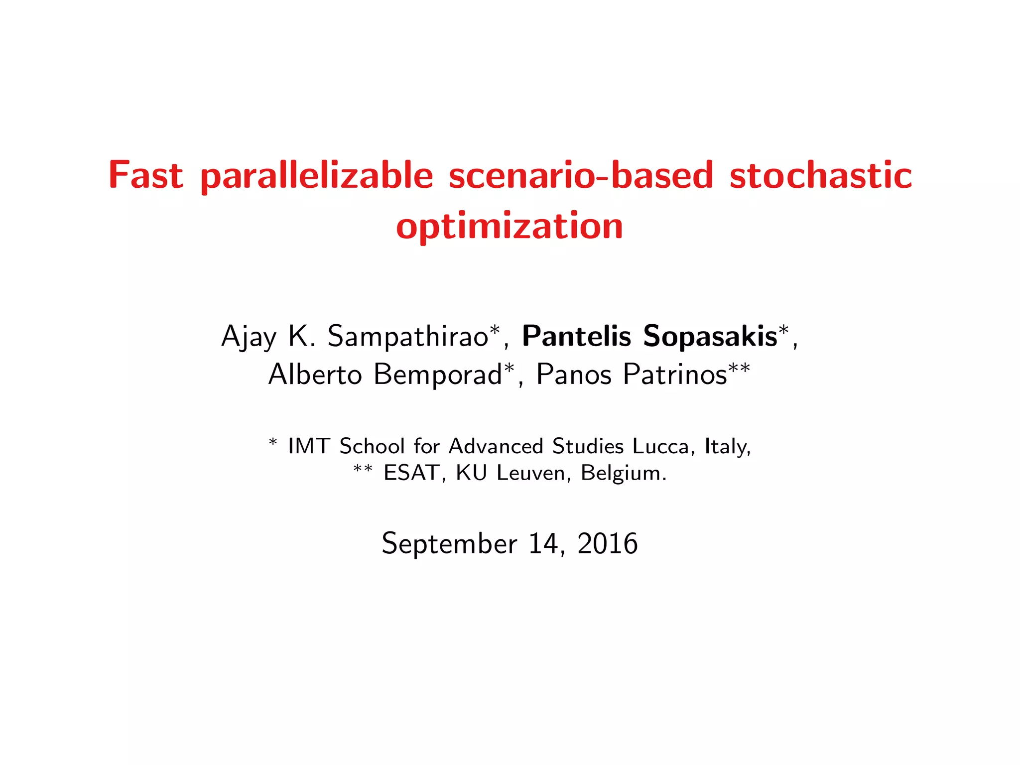
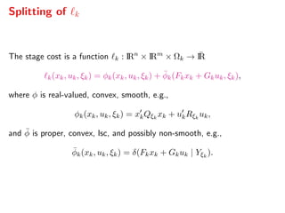
Optimisation problem:
V (p) = min
π={uk}k=N−1
k=0
E Vf (xN , ξN ) +
N−1
k=0
k(xk, uk, ξk) ,
s.t x0 = p,
xk+1 = Aξk
xk + Bξk
uk + wξk
,
where:
At time k we measure xk and ξk−1
E[·]: conditional expectation wrt the product probability measure
Sampathirao et al., 2015, 2016.](https://image.slidesharecdn.com/sopasakis-eucco-2016-160914140648/85/Fast-parallelizable-scenario-based-stochastic-optimization-5-320.jpg)
![Stochastic Optimal Control
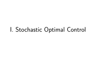
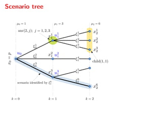
Optimisation problem:
V (p) = min
π={uk}k=N−1
k=0
E Vf (xN , ξN ) +
N−1
k=0
k(xk, uk, ξk) ,
s.t x0 = p,
xk+1 = Aξk
xk + Bξk
uk + wξk
,
where:
At time k we measure xk and ξk−1
E[·]: conditional expectation wrt the product probability measure
Casual policy uk = ψk(p,ξξξk−1), with ξξξk = (ξ0, ξ1, . . . , ξk)
Sampathirao et al., 2015, 2016.](https://image.slidesharecdn.com/sopasakis-eucco-2016-160914140648/85/Fast-parallelizable-scenario-based-stochastic-optimization-6-320.jpg)
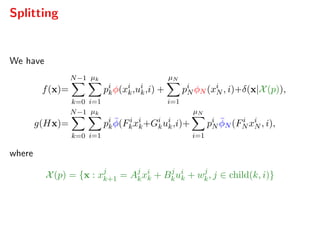
![Stochastic Optimal Control
Optimisation problem:
V (p) = min
π={uk}k=N−1
k=0
E Vf (xN , ξN ) +
N−1
k=0
k(xk, uk, ξk) ,
s.t x0 = p,
xk+1 = Aξk
xk + Bξk
uk + wξk
,
where:
At time k we measure xk and ξk−1
E[·]: conditional expectation wrt the product probability measure
Casual policy uk = ψk(p,ξξξk−1), with ξξξk = (ξ0, ξ1, . . . , ξk)
and Vf can encode constraints
Sampathirao et al., 2015, 2016.](https://image.slidesharecdn.com/sopasakis-eucco-2016-160914140648/85/Fast-parallelizable-scenario-based-stochastic-optimization-7-320.jpg)
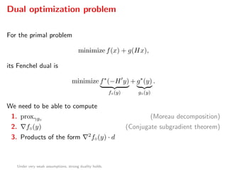

![Dual gradient
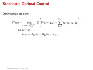
Algorithm 3 Dual gradient computation
Input: y, Factorization matrices
Output: x∗ = {xi
k, ui
k}, so that f◦(y) = Hx∗
1: qi
N ← yi
N , ∀i ∈ N[1,µN ], x1
0 ← p
2: for k = N − 1, . . . , 0 do
3: for i = 1, . . . , µk do in parallel
4: ui
k ← Φi
kyi
k + j∈child(k,i) Θj
kqj
k+1 + σi
k matvec only
5: qi
k ← Di
k yi
k + j∈child(k,i) Λj
k qj
k+1 + ci
k
6: for k = 0, . . . , N − 1 do
7: for i = 1, . . . , µk do in parallel
8: ui
k ← Ki
kxi
k + ui
k
9: for j ∈ child(k, i) do in parallel
10: xj
k+1 ← Aj
kxi
k + Bj
kui
k + wj
k](https://image.slidesharecdn.com/sopasakis-eucco-2016-160914140648/85/Fast-parallelizable-scenario-based-stochastic-optimization-29-320.jpg)
![Hessian-vector products
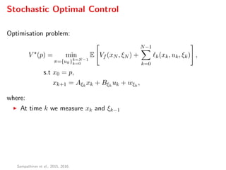
Algorithm 4 Computation of Hessian-vector products
Input: Vector d
Output: {ˆxi
k, ˆui
k} = 2f◦(y)d
1: ˆqi
N ← di
N , ∀i ∈ N[1,µN ], ˆx1
0 ← 0
2: for k = N − 1, . . . , 0 do
3: for i = 1, . . . , µk do in parallel
4: ˆui
k ← Φi
kdi
k + j∈child(k,i) Θj
k ˆqj
k+1 matvec only
5: ˆqi
k ← Di
k di
k + j∈child(k,i) Λj
k ˆqj
k+1
6: for k = 0, . . . , N − 1 do
7: for i = 1, . . . , µk do in parallel
8: ui
k ← Ki
k ˆxi
k + ˆui
k
9: for j ∈ child(k, i) do in parallel
10: ˆxj
k+1 ← Aj
k ˆxi
k + Bj
k ˆui
k](https://image.slidesharecdn.com/sopasakis-eucco-2016-160914140648/85/Fast-parallelizable-scenario-based-stochastic-optimization-30-320.jpg)

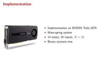
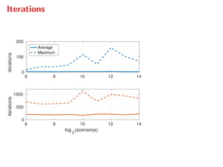


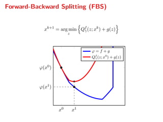
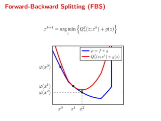
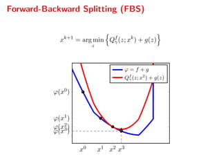
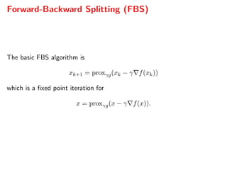
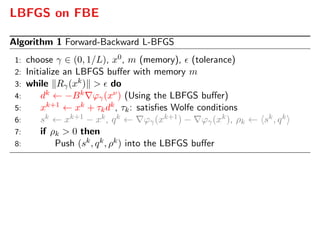
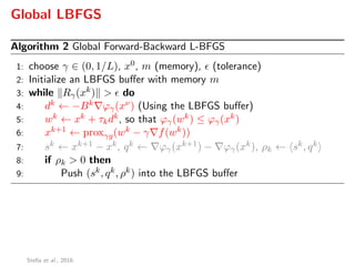
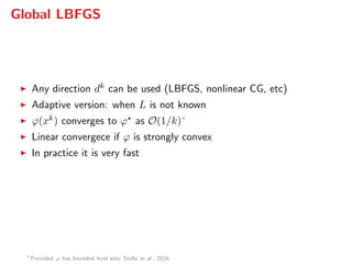
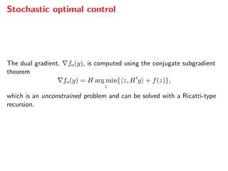
The document presents a comprehensive study on fast parallelizable scenario-based stochastic optimization, focusing on stochastic optimal control problems, their formulations, and solution methods. It includes discussions about the forward-backward line-search algorithm, dual gradient algorithms, and Hessian-vector product computations, showcasing their implementations and results using NVIDIA GPUs. The work aims to enhance computational efficiency in solving complex optimization problems across various applications.