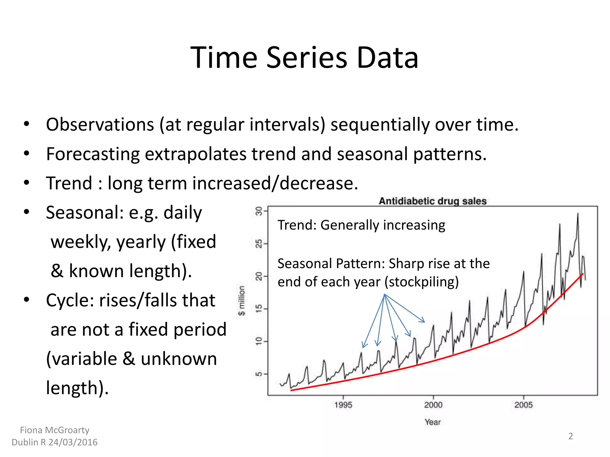
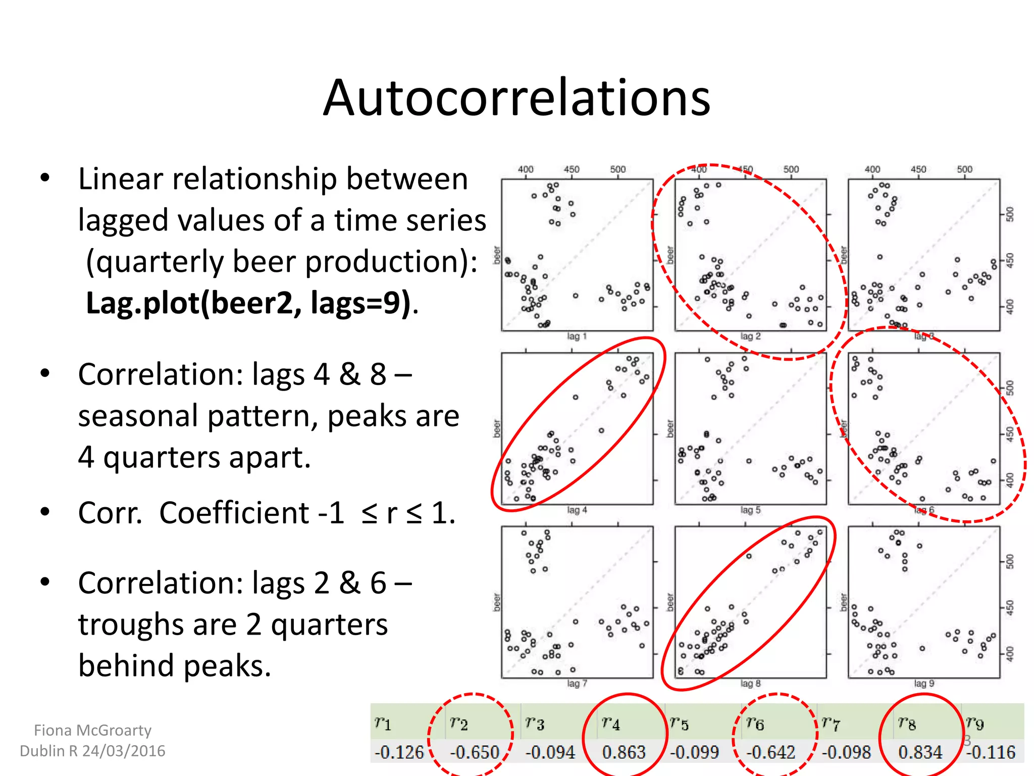
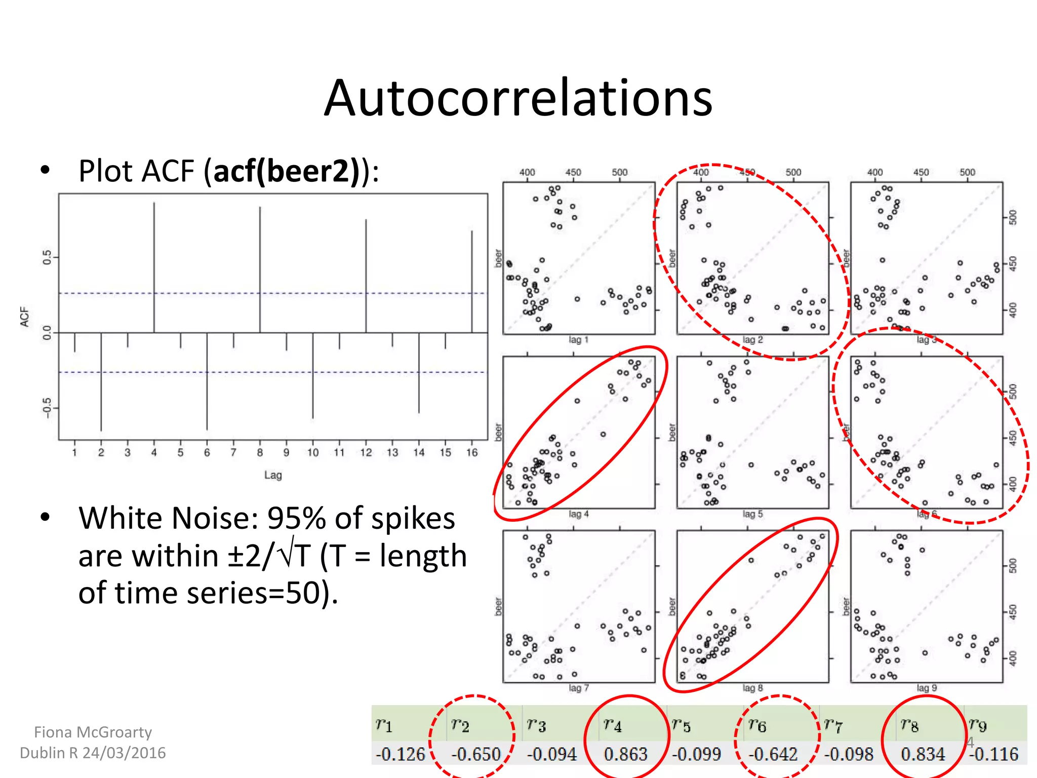
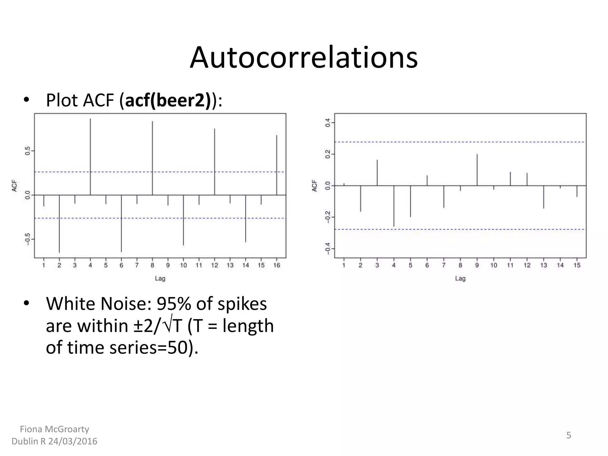
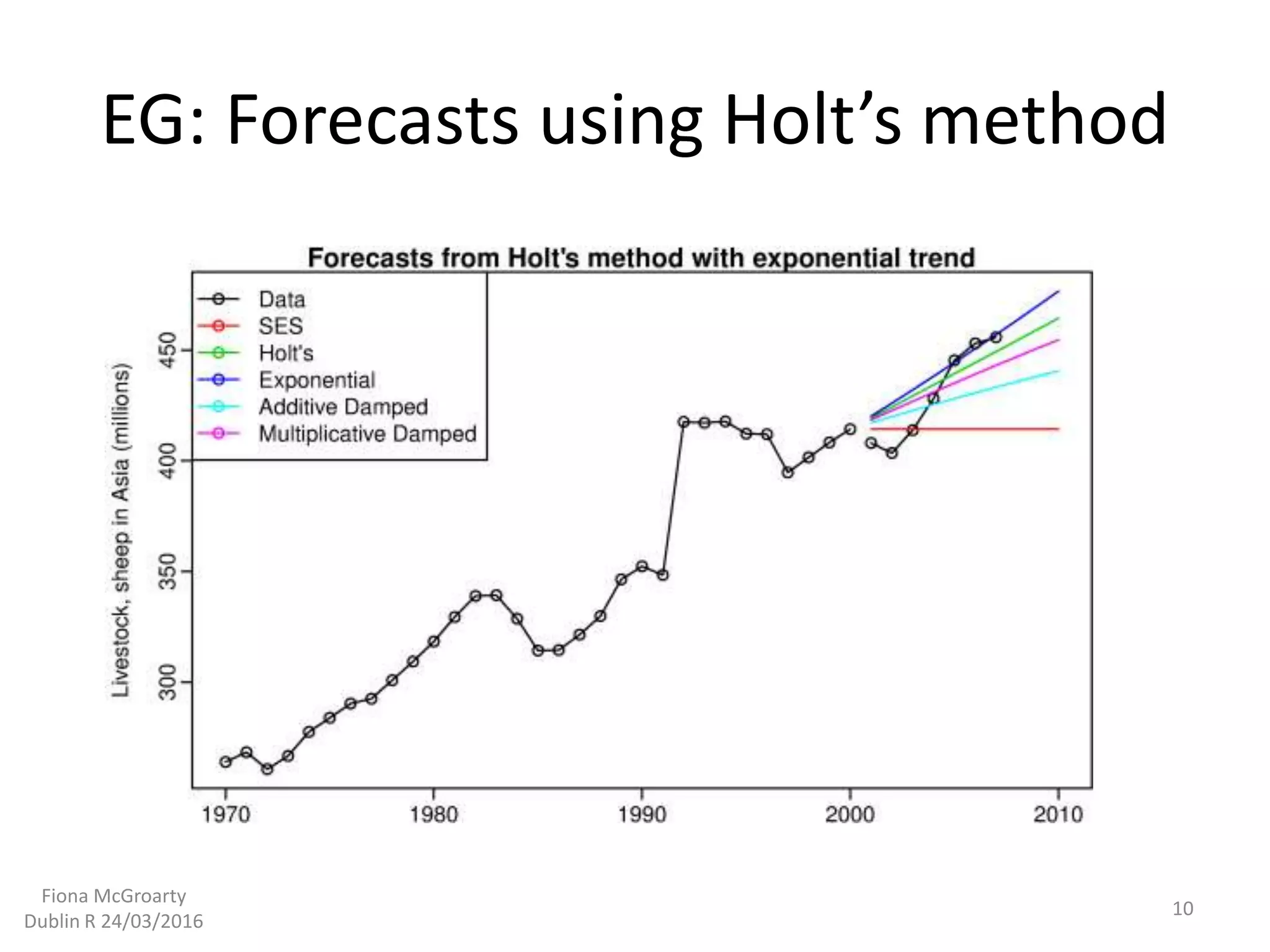
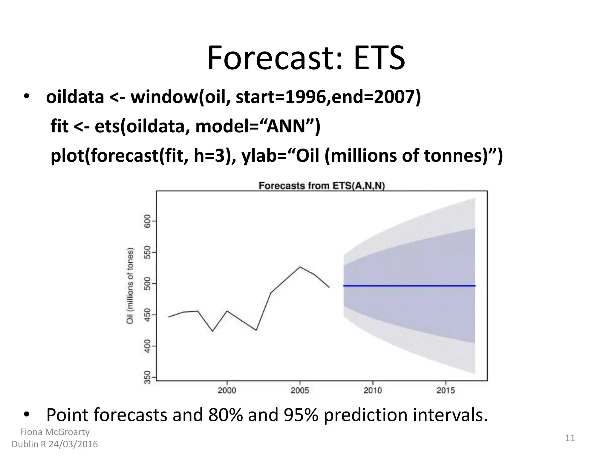
Time Series Analysis & fpp
• Used to predict wind speeds at forecast horizons of 10
minutes to 1 day ahead, based on historical wind speeds (10
minute averages).
• Forecast package: Rob Hyndman
• https://www.otexts.org/fpp - good explanations and worked
examples.
1
Fiona McGroarty
Dublin R 24/03/2016
Time Series Data
• Forecasting extrapolates trend and seasonal patterns.
• Trend : long term increased/decrease.
• Seasonal: e.g. daily
weekly, yearly (fixed
& known length).
• Cycle: rises/falls that
are not a fixed period
(variable & unknown
length).
Trend: Generally increasing
Seasonal Pattern: Sharp rise at the
end of each year (stockpiling)
• Observations (at regular intervals) sequentially over time.
2
Fiona McGroarty
Dublin R 24/03/2016
Autocorrelations
• Correlation: lags 4 & 8 –
seasonal pattern, peaks are
4 quarters apart.
• Linear relationship between
lagged values of a time series
(quarterly beer production):
Lag.plot(beer2, lags=9).
• Corr. Coefficient -1 ≤ r ≤ 1.
• Correlation: lags 2 & 6 –
troughs are 2 quarters
behind peaks.
3
Fiona McGroarty
Dublin R 24/03/2016
Autocorrelations
• Plot ACF (acf(beer2)):
• White Noise: 95% of spikes
are within ±2/T (T = length
of time series=50).
4
Fiona McGroarty
Dublin R 24/03/2016
Autocorrelations
• Plot ACF (acf(beer2)):
• White Noise: 95% of spikes
are within ±2/T (T = length
of time series=50).
5
Fiona McGroarty
Dublin R 24/03/2016
Simple Forecasts (Benchmarks)
• Naïve method: forecast = value of last observation:
naive(beer2, h=11) or rwf(beer2, h=11).
• Average method: forecast = mean of historical data:
meanf(beer2, h=11).
• Seasonal naïve: forecast = value of last observation from the
previous season
(month/quarter/year ...)
snaive(beer2, h=11).
6
Fiona McGroarty
Dublin R 24/03/2016
Simple Forecasts (Benchmarks)
• Drift: variation on naïve, allow forecast to increase/decrease
over time: rwf (dj2, h=42, drift=TRUE)
7
Fiona McGroarty
Dublin R 24/03/2016
Time Series Decomposition
• fit <- stl (elecequip,
t.window=15,
s.window=“periodic”,
robust=TRUE).
Plot(fit).
• Time series decomposition: yt = St + Tt + Et or yt = St × Tt × Et
Electrical equipment orders. (Seasonal, Trend, Error)
• Set trend window and seasonal
window sizes – small values
allow more rapid changes.
8
Fiona McGroarty
Dublin R 24/03/2016
Forecast: ETS
• Effects of components can be additive (A), multiplicative (M) or
ignored (N, none). EG ETS (MAN) forecasts by multiplying errors
(M), adding trends (A) and ignoring seasonal effects (N).
SES: Simple Exponential Smoothing
Holts Linear Method
Additive Holts-Winter Method
Multiplicative Holts-Winter Method
Holts-Winter damped method
• ETS (ANN) SES with + errors; ETS (MNN) SES with × errors.
• Some are numerically unstable e.g. if data contains 0 or neg. values.
• ETS(ZZZ) – runs all (stable) ETS models and returns the optimal one.
• ETS (Error, Trend, Seasonal OR ExponenTial Smoothing)
9
Fiona McGroarty
Dublin R 24/03/2016
EG: Forecasts using Holt’s method
10
Fiona McGroarty
Dublin R 24/03/2016
Forecast: ETS
• oildata <- window(oil, start=1996,end=2007)
fit <- ets(oildata, model=“ANN”)
plot(forecast(fit, h=3), ylab=“Oil (millions of tonnes)”)
• Point forecasts and 80% and 95% prediction intervals.
11
Fiona McGroarty
Dublin R 24/03/2016
ARIMA Models
• ARIMA (p, d, q) e.g. ARIMA101 model uses one past time-
lagged wind speed autocorrelation term (p = 1), is not
differentiated (d = 0) and uses one past forecast error (q = 1).
• ARIMA = Auto Regression (detects similarity in the data using
timelagged values of the variable) Integrated (the data may
have to be differentiated a number of times to make it
stationary) Moving Average (using weighted moving average
of the past few forecast errors).
• Can specify the ARIMA (p, d, q) model to use, or use
auto.arima
12
Fiona McGroarty
Dublin R 24/03/2016
ARIMA Models
• fit <- auto.arima (usconsumption[,1], seasonal=FALSE
plot(forecast(fit, h=10), include=80)
• Best ARIMA model is returned, in this case it’s ARIMA(0,0,3).
• fit <- Arima(usconsumption[,1], order=c(0,0,3))
13
Fiona McGroarty
Dublin R 24/03/2016
Lots of other things to consider….
• Stationarity of data
• Transforming data before forecasting – differentiating…
• Error Metrics! Calculate MAE, RMSE,…..
14
Fiona McGroarty
Dublin R 24/03/2016

Time series Analysis & fpp package

  • 1.
    Time Series Analysis& fpp • Used to predict wind speeds at forecast horizons of 10 minutes to 1 day ahead, based on historical wind speeds (10 minute averages). • Forecast package: Rob Hyndman • https://www.otexts.org/fpp - good explanations and worked examples. 1 Fiona McGroarty Dublin R 24/03/2016
  • 2.
    Time Series Data •Forecasting extrapolates trend and seasonal patterns. • Trend : long term increased/decrease. • Seasonal: e.g. daily weekly, yearly (fixed & known length). • Cycle: rises/falls that are not a fixed period (variable & unknown length). Trend: Generally increasing Seasonal Pattern: Sharp rise at the end of each year (stockpiling) • Observations (at regular intervals) sequentially over time. 2 Fiona McGroarty Dublin R 24/03/2016
  • 3.
    Autocorrelations • Correlation: lags4 & 8 – seasonal pattern, peaks are 4 quarters apart. • Linear relationship between lagged values of a time series (quarterly beer production): Lag.plot(beer2, lags=9). • Corr. Coefficient -1 ≤ r ≤ 1. • Correlation: lags 2 & 6 – troughs are 2 quarters behind peaks. 3 Fiona McGroarty Dublin R 24/03/2016
  • 4.
    Autocorrelations • Plot ACF(acf(beer2)): • White Noise: 95% of spikes are within ±2/T (T = length of time series=50). 4 Fiona McGroarty Dublin R 24/03/2016
  • 5.
    Autocorrelations • Plot ACF(acf(beer2)): • White Noise: 95% of spikes are within ±2/T (T = length of time series=50). 5 Fiona McGroarty Dublin R 24/03/2016
  • 6.
    Simple Forecasts (Benchmarks) •Naïve method: forecast = value of last observation: naive(beer2, h=11) or rwf(beer2, h=11). • Average method: forecast = mean of historical data: meanf(beer2, h=11). • Seasonal naïve: forecast = value of last observation from the previous season (month/quarter/year ...) snaive(beer2, h=11). 6 Fiona McGroarty Dublin R 24/03/2016
  • 7.
    Simple Forecasts (Benchmarks) •Drift: variation on naïve, allow forecast to increase/decrease over time: rwf (dj2, h=42, drift=TRUE) 7 Fiona McGroarty Dublin R 24/03/2016
  • 8.
    Time Series Decomposition •fit <- stl (elecequip, t.window=15, s.window=“periodic”, robust=TRUE). Plot(fit). • Time series decomposition: yt = St + Tt + Et or yt = St × Tt × Et Electrical equipment orders. (Seasonal, Trend, Error) • Set trend window and seasonal window sizes – small values allow more rapid changes. 8 Fiona McGroarty Dublin R 24/03/2016
  • 9.
    Forecast: ETS • Effectsof components can be additive (A), multiplicative (M) or ignored (N, none). EG ETS (MAN) forecasts by multiplying errors (M), adding trends (A) and ignoring seasonal effects (N). SES: Simple Exponential Smoothing Holts Linear Method Additive Holts-Winter Method Multiplicative Holts-Winter Method Holts-Winter damped method • ETS (ANN) SES with + errors; ETS (MNN) SES with × errors. • Some are numerically unstable e.g. if data contains 0 or neg. values. • ETS(ZZZ) – runs all (stable) ETS models and returns the optimal one. • ETS (Error, Trend, Seasonal OR ExponenTial Smoothing) 9 Fiona McGroarty Dublin R 24/03/2016
  • 10.
    EG: Forecasts usingHolt’s method 10 Fiona McGroarty Dublin R 24/03/2016
  • 11.
    Forecast: ETS • oildata<- window(oil, start=1996,end=2007) fit <- ets(oildata, model=“ANN”) plot(forecast(fit, h=3), ylab=“Oil (millions of tonnes)”) • Point forecasts and 80% and 95% prediction intervals. 11 Fiona McGroarty Dublin R 24/03/2016
  • 12.
    ARIMA Models • ARIMA(p, d, q) e.g. ARIMA101 model uses one past time- lagged wind speed autocorrelation term (p = 1), is not differentiated (d = 0) and uses one past forecast error (q = 1). • ARIMA = Auto Regression (detects similarity in the data using timelagged values of the variable) Integrated (the data may have to be differentiated a number of times to make it stationary) Moving Average (using weighted moving average of the past few forecast errors). • Can specify the ARIMA (p, d, q) model to use, or use auto.arima 12 Fiona McGroarty Dublin R 24/03/2016
  • 13.
    ARIMA Models • fit<- auto.arima (usconsumption[,1], seasonal=FALSE plot(forecast(fit, h=10), include=80) • Best ARIMA model is returned, in this case it’s ARIMA(0,0,3). • fit <- Arima(usconsumption[,1], order=c(0,0,3)) 13 Fiona McGroarty Dublin R 24/03/2016
  • 14.
    Lots of otherthings to consider…. • Stationarity of data • Transforming data before forecasting – differentiating… • Error Metrics! Calculate MAE, RMSE,….. 14 Fiona McGroarty Dublin R 24/03/2016