Robustness and Regularization of Support Vector Machines.pdf

Journal of Machine Learning Research 10 (2009) 1485-1510 Submitted 3/08; Revised 10/08; Published 7/09
Robustness and Regularization of Support Vector Machines
Huan Xu XUHUAN@CIM.MCGILL.CA
Department of Electrical and Computer Engineering
3480 University Street
McGill University
Montreal, Canada H3A 2A7
Constantine Caramanis CARAMANIS@MAIL.UTEXAS.EDU
The University of Texas at Austin
1 University Station C0803
Austin, TX, 78712, USA
Shie Mannor∗ SHIE.MANNOR@MCGILL.CA
3480 University Street
McGill University
Montreal, Canada H3A 2A7
Editor: Alexander Smola
Abstract
We consider regularized support vector machines (SVMs) and show that they are precisely equiva-
lent to a new robust optimization formulation. We show that this equivalence of robust optimization
and regularization has implications for both algorithms, and analysis. In terms of algorithms, the
equivalence suggests more general SVM-like algorithms for classification that explicitly build in
protection to noise, and at the same time control overfitting. On the analysis front, the equiva-
lence of robustness and regularization provides a robust optimization interpretation for the success
of regularized SVMs. We use this new robustness interpretation of SVMs to give a new proof of
consistency of (kernelized) SVMs, thus establishing robustness as the reason regularized SVMs
generalize well.
Keywords: robustness, regularization, generalization, kernel, support vector machine
1. Introduction
Support Vector Machines (SVMs for short) originated in Boser et al. (1992) and can be traced back
to as early as Vapnik and Lerner (1963) and Vapnik and Chervonenkis (1974). They continue to be
one of the most successful algorithms for classification. SVMs address the classification problem by
finding the hyperplane in the feature space that achieves maximum sample margin when the training
samples are separable, which leads to minimizing the norm of the classifier. When the samples are
not separable, a penalty term that approximates the total training error is considered (Bennett and
Mangasarian, 1992; Cortes and Vapnik, 1995). It is well known that minimizing the training error
itself can lead to poor classification performance for new unlabeled data; that is, such an approach
∗. Also at the Department of Electrical Engineering, Technion, Israel.
c 2009 Huan Xu, Constantine Caramanis and Shie Mannor.

XU, CARAMANIS AND MANNOR
may have poor generalization error because of, essentially, overfitting (Vapnik and Chervonenkis,
1991). A variety of modifications have been proposed to handle this, one of the most popular
methods being that of minimizing a combination of the training-error and a regularization term. The
latter is typically chosen as a norm of the classifier. The resulting regularized classifier performs
better on new data. This phenomenon is often interpreted from a statistical learning theory view:
the regularization term restricts the complexity of the classifier, hence the deviation of the testing
error and the training error is controlled (see Smola et al., 1998; Evgeniou et al., 2000; Bartlett and
Mendelson, 2002; Koltchinskii and Panchenko, 2002; Bartlett et al., 2005, and references therein).
In this paper we consider a different setup, assuming that the training data are generated by
the true underlying distribution, but some non-i.i.d. (potentially adversarial) disturbance is then
added to the samples we observe. We follow a robust optimization (see El Ghaoui and Lebret,
1997; Ben-Tal and Nemirovski, 1999; Bertsimas and Sim, 2004, and references therein) approach,
that is, minimizing the worst possible empirical error under such disturbances. The use of robust
optimization in classification is not new (e.g., Shivaswamy et al., 2006; Bhattacharyya et al., 2004b;
Lanckriet et al., 2003), in which box-type uncertainty sets were considered. Moreover, there has
not been an explicit connection to the regularized classifier, although at a high-level it is known that
regularization and robust optimization are related (e.g., El Ghaoui and Lebret, 1997; Anthony and
Bartlett, 1999). The main contribution in this paper is solving the robust classification problem for
a class of non-box-typed uncertainty sets, and providing a linkage between robust classification and
the standard regularization scheme of SVMs. In particular, our contributions include the following:
• We solve the robust SVM formulation for a class of non-box-type uncertainty sets. This per-
mits finer control of the adversarial disturbance, restricting it to satisfy aggregate constraints
across data points, therefore reducing the possibility of highly correlated disturbance.
• We show that the standard regularized SVM classifier is a special case of our robust clas-
sification, thus explicitly relating robustness and regularization. This provides an alternative
explanation to the success of regularization, and also suggests new physically motivated ways
to construct regularization terms.
• We relate our robust formulation to several probabilistic formulations. We consider a chance-
constrained classifier (that is, a classifier with probabilistic constraints on misclassification)
and show that our robust formulation can approximate it far less conservatively than previous
robust formulations could possibly do. We also consider a Bayesian setup, and show that this
can be used to provide a principled means of selecting the regularization coefficient without
cross-validation.
• We show that the robustness perspective, stemming from a non-i.i.d. analysis, can be useful
in the standard learning (i.i.d.) setup, by using it to prove consistency for standard SVM
classification, without using VC-dimension or stability arguments. This result implies that
generalization ability is a direct result of robustness to local disturbances; it therefore suggests
a new justification for good performance, and consequently allows us to construct learning
algorithms that generalize well by robustifying non-consistent algorithms.
1486

ROBUSTNESS AND REGULARIZATION OF SVMS
1.1 Robustness and Regularization
We comment here on the explicit equivalence of robustness and regularization. We briefly explain
how this observation is different from previous work and why it is interesting. Previous works on
robust classification (e.g., Lanckriet et al., 2003; Bhattacharyya et al., 2004a,b; Shivaswamy et al.,
2006; Trafalis and Gilbert, 2007) consider robustifying regularized classifications.1 That is, they
propose modifications to standard regularized classifications so that the new formulations are robust
to input uncertainty. Furthermore, box-type uncertainty—a setup where the joint uncertainty is the
Cartesian product of uncertainty in each input (see Section 2 for detailed formulation)—is consid-
ered, which leads to penalty terms on each constraint of the resulting formulation. The objective
of these works was not to relate robustness and the standard regularization term that appears in the
objective function. Indeed, research on classifier regularization mainly considers its effect on bound-
ing the complexity of the function class (e.g., Smola et al., 1998; Evgeniou et al., 2000; Bartlett and
Mendelson, 2002; Koltchinskii and Panchenko, 2002; Bartlett et al., 2005). Thus, although certain
equivalence relationships between robustness and regularization have been established for problems
other than classification (El Ghaoui and Lebret, 1997; Ben-Tal and Nemirovski, 1999; Bishop, 1995;
Xu et al., 2009), the explicit equivalence between robustness and regularization in the SVM setup
is novel.
The connection of robustness and regularization in the SVM context is important for the follow-
ing reasons. First, it gives an alternative and potentially powerful explanation of the generalization
ability of the regularization term. In the standard machine learning view, the regularization term
bounds the complexity of the class of classifiers. The robust view of regularization regards the test-
ing samples as a perturbed copy of the training samples. Therefore, when the total perturbation is
given or bounded, the regularization term bounds the gap between the classification errors of the
SVM on these two sets of samples. In contrast to the standard PAC approach, this bound depends
neither on how rich the class of candidate classifiers is, nor on an assumption that all samples are
picked in an i.i.d. manner.
Second, this connection suggests novel approaches to designing good classification algorithms,
in particular, designing the regularization term. In the PAC structural-risk minimization approach,
regularization is chosen to minimize a bound on the generalization error based on the training error
and a complexity term. This approach is known to often be too pessimistic (Kearns et al., 1997),
especially for problems with more structure. The robust approach offers another avenue. Since
both noise and robustness are physical processes, a close investigation of the application and noise
characteristics at hand, can provide insights into how to properly robustify, and therefore regularize
the classifier. For example, it is known that normalizing the samples so that the variance among all
features is roughly the same (a process commonly used to eliminate the scaling freedom of individ-
ual features) often leads to good generalization performance. From the robustness perspective, this
has the interpretation that the noise is anisotropic (ellipsoidal) rather than spherical, and hence an
appropriate robustification must be designed to fit this anisotropy.
We also show that using the robust optimization viewpoint, we obtain some probabilistic results
that go beyond the PAC setup. In Section 3 we bound the probability that a noisy training sample is
correctly labeled. Such a bound considers the behavior of corrupted samples and is hence different
from the known PAC bounds. This is helpful when the training samples and the testing samples are
1. Lanckriet et al. (2003) is perhaps the only exception, where a regularization term is added to the covariance estimation
rather than to the objective function.
1487

drawn from different distributions, or some adversary manipulates the samples to prevent them from
being correctly labeled (e.g., spam senders change their patterns from time to time to avoid being
labeled and filtered). Finally, this connection of robustification and regularization also provides us
with new proof techniques as well (see Section 5).
We need to point out that there are several different definitions of robustness in the literature. In
this paper, as well as the aforementioned robust classification papers, robustness is mainly under-
stood from a Robust Optimization (RO) perspective, where a min-max optimization is performed
over all possible disturbances. An alternative interpretation of robustness stems from the rich lit-
erature on robust statistics (e.g., Huber, 1981; Hampel et al., 1986; Rousseeuw and Leroy, 1987;
Maronna et al., 2006), which studies how an estimator or algorithm behaves under a small pertur-
bation of the statistics model. For example, the influence function approach, proposed in Hampel
(1974) and Hampel et al. (1986), measures the impact of an infinitesimal amount of contamination
of the original distribution on the quantity of interest. Based on this notion of robustness, Christ-
mann and Steinwart (2004) showed that many kernel classification algorithms, including SVM, are
robust in the sense of having a finite Influence Function. A similar result for regression algorithms
is shown in Christmann and Steinwart (2007) for smooth loss functions, and in Christmann and Van
Messem (2008) for non-smooth loss functions where a relaxed version of the Influence Function is
applied. In the machine learning literature, another widely used notion closely related to robustness
is the stability, where an algorithm is required to be robust (in the sense that the output function does
not change significantly) under a specific perturbation: deleting one sample from the training set. It
is now well known that a stable algorithm such as SVM has desirable generalization properties, and
is statistically consistent under mild technical conditions; see for example Bousquet and Elisseeff
(2002), Kutin and Niyogi (2002), Poggio et al. (2004) and Mukherjee et al. (2006) for details. One
main difference between RO and other robustness notions is that the former is constructive rather
than analytical. That is, in contrast to robust statistics or the stability approach that measures the
robustness of a given algorithm, RO can robustify an algorithm: it converts a given algorithm to
a robust one. For example, as we show in this paper, the RO version of a naive empirical-error
minimization is the well known SVM. As a constructive process, the RO approach also leads to
additional flexibility in algorithm design, especially when the nature of the perturbation is known
or can be well estimated.
1.2 Structure of the Paper
This paper is organized as follows. In Section 2 we investigate the correlated disturbance case, and
show the equivalence between the robust classification and the regularization process. We develop
the connections to probabilistic formulations in Section 3. The kernelized version is investigated
in Section 4. Finally, in Section 5, we consider the standard statistical learning setup where all
samples are i.i.d. draws and provide a novel proof of consistency of SVM based on robustness
analysis. The analysis shows that duplicate copies of iid draws tend to be “similar” to each other
in the sense that with high probability the total difference is small, and hence robustification that
aims to control performance loss for small perturbations can help mitigate overfitting even though
no explicit perturbation exists.
1488

1.3 Notation
Capital letters are used to denote matrices, and boldface letters are used to denote column vectors.
For a given norm k·k, we use k·k∗ to denote its dual norm, that is, kzk∗ , sup{z⊤x|kxk ≤ 1}. For
a vector x and a positive semi-definite matrix C of the same dimension, kxkC denotes
√
x⊤Cx. We
use δ to denote disturbance affecting the samples. We use superscript r to denote the true value
for an uncertain variable, so that δr
i is the true (but unknown) noise of the ith sample. The set of
non-negative scalars is denoted by R+. The set of integers from 1 to n is denoted by [1 : n].
2. Robust Classification and Regularization
We consider the standard binary classification problem, where we are given a finite number of
training samples {xi,yi}m
i=1 ⊆ Rn × {−1,+1}, and must find a linear classifier, specified by the
function hw,b(x) = sgn(hw, xi+b). For the standard regularized classifier, the parameters (w,b) are
obtained by solving the following convex optimization problem:
min
w,b,ξ
: r(w,b)+
m
∑
i=1
ξi
s.t. : ξi ≥

1−yi(hw,xii+b)]
ξi ≥ 0,
where r(w,b) is a regularization term. This is equivalent to
min
w,b
(
r(w,b)+
m
∑
i=1
max

1−yi(hw,xii+b),0

)
.
Previous robust classification work (Shivaswamy et al., 2006; Bhattacharyya et al., 2004a,b; Bhat-
tacharyya, 2004; Trafalis and Gilbert, 2007) considers the classification problem where the input
are subject to (unknown) disturbances ~
δ = (δ1,...,δm) and essentially solves the following min-
max problem:
min
w,b
max
~
δ∈Nbox
(
r(w,b)+
m
∑
i=1
max

1−yi(hw, xi −δii+b),0

)
, (1)
for a box-type uncertainty set Nbox. That is, let Ni denote the projection of Nbox onto the δi com-
ponent, then Nbox = N1 × ··· × Nm (note that Ni need not be a “box”). Effectively, this allows
simultaneous worst-case disturbances across many samples, and leads to overly conservative solu-
tions. The goal of this paper is to obtain a robust formulation where the disturbances {δi} may be
meaningfully taken to be correlated, that is, to solve for a non-box-type N :
min
w,b
max
~
δ∈N
(
r(w,b)+
m
∑
i=1
max

1−yi(hw,xi −δii+b),0

)
. (2)
We briefly explain here the four reasons that motivate this “robust to perturbation” setup and in par-
ticular the min-max form of (1) and (2). First, it can explicitly incorporate prior problem knowledge
of local invariance (e.g., Teo et al., 2008). For example, in vision tasks, a desirable classifier should
provide a consistent answer if an input image slightly changes. Second, there are situations where
1489

some adversarial opponents (e.g., spam senders) will manipulate the testing samples to avoid being
correctly classified, and the robustness toward such manipulation should be taken into consideration
in the training process (e.g., Globerson and Roweis, 2006). Or alternatively, the training samples
and the testing samples can be obtained from different processes and hence the standard i.i.d. as-
sumption is violated (e.g., Bi and Zhang, 2004). For example in real-time applications, the newly
generated samples are often less accurate due to time constraints. Finally, formulations based on
chance-constraints (e.g., Bhattacharyya et al., 2004b; Shivaswamy et al., 2006) are mathematically
equivalent to such a min-max formulation.
We define explicitly the correlated disturbance (or uncertainty) which we study below.
Definition 1 A set N0 ⊆ Rn is called an Atomic Uncertainty Set if
(I) 0 ∈ N0;
(II) For any w0 ∈ Rn
: sup
δ∈N0
[w⊤
0 δ] = sup
δ′
∈N0
[−w⊤
0 δ′
] +∞.
We use “sup” here because the maximal value is not necessary attained since N0 may not be a
closed set. The second condition of Atomic Uncertainty set basically says that the uncertainty set is
bounded and symmetric. In particular, all norm balls and ellipsoids centered at the origin are atomic
uncertainty sets, while an arbitrary polytope might not be an atomic uncertainty set.
Definition 2 Let N0 be an atomic uncertainty set. A set N ⊆ Rn×m is called a Sublinear Aggregated
Uncertainty Set of N0, if
N −
⊆ N ⊆ N +
,
where: N −
,
m
[
t=1
N −
t ; N −
t , {(δ1,··· ,δm)|δt ∈ N0; δi6=t = 0}.
N +
, {(α1δ1,··· ,αmδm)|
m
∑
i=1
αi = 1; αi ≥ 0, δi ∈ N0, i = 1,··· ,m}.
The Sublinear Aggregated Uncertainty definition models the case where the disturbances on each
sample are treated identically, but their aggregate behavior across multiple samples is controlled.
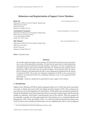
Some interesting examples include
(1) {(δ1,··· ,δm)|
m
∑
i=1
kδik ≤ c};
(2) {(δ1,··· ,δm)|∃t ∈ [1 : m]; kδtk ≤ c; δi = 0,∀i 6= t};
(3) {(δ1,··· ,δm)|
m
∑
i=1
p
ckδik ≤ c}.
All these examples have the same atomic uncertainty set N0 =

δ kδk ≤ c . Figure 1 provides an
illustration of a sublinear aggregated uncertainty set for n = 1 and m = 2, that is, the training set
consists of two univariate samples.
The following theorem is the main result of this section, which reveals that standard norm reg-
ularized SVM is the solution of a (non-regularized) robust optimization. It is a special case of
Proposition 4 by taking N0 as the dual-norm ball {δ|kδk∗ ≤ c} for an arbitrary norm k · k and
r(w,b) ≡ 0.
1490

xxxxxxxxxxxxxxxxxxxxxxxxxxxxxxxxxxxxxxxxxxxxxxxxxxxxxxxxx
xxxxxxxxxxxxxxxxxxxxxxxxxxxxxxxxxxxxxxxxxxxxxxxxxxxxx
xxxxxxxxxxxxxxxxxxxxxxxxxxxxx
a. N − b. N + c. N d. Box uncertainty
Figure 1: Illustration of a Sublinear Aggregated Uncertainty Set N .
Theorem 3 Let T ,
n
(δ1,···δm)|∑m
i=1 kδik∗ ≤ c
o
. Suppose that the training sample {xi,yi}m
i=1
are non-separable. Then the following two optimization problems on (w,b) are equivalent2
min : max
(δ1,···,δm)∈T
m
∑
i=1
max

1−yi hw, xi −δii+b

,0

,
min : ckwk+
m
∑
i=1
max

1−yi hw, xii+b

,0

.
(3)
Proposition 4 Assume {xi,yi}m
i=1 are non-separable, r(·) : Rn+1 → R is an arbitrary function, N
is a Sublinear Aggregated Uncertainty set with corresponding atomic uncertainty set N0. Then the
following min-max problem
min
w,b
sup
(δ1,···,δm)∈N
n
r(w,b)+
m
∑
i=1
max

1−yi(hw,xi −δii+b), 0
o
(4)
is equivalent to the following optimization problem on w,b,ξ:
min : r(w,b)+ sup
δ∈N0
(w⊤
δ)+
m
∑
i=1
ξi,
s.t. : ξi ≥ 1−[yi(hw, xii+b)], i = 1,...,m;
ξi ≥ 0, i = 1,...,m.
(5)
Furthermore, the minimization of Problem (5) is attainable when r(·,·) is lower semi-continuous.
Proof Define:
v(w,b) , sup
δ∈N0
(w⊤
δ)+
m
∑
i=1
max

1−yi(hw,xii+b), 0

.
2. The optimization equivalence for the linear case was observed independently by Bertsimas and Fertis (2008).
1491

Recall that N − ⊆ N ⊆ N+ by definition. Hence, fixing any (ŵ,b̂) ∈ Rn+1, the following inequalities
hold:
sup
(δ1,···,δm)∈N −
m
∑
i=1
max

1−yi(hŵ,xi −δii+b̂), 0

≤ sup
(δ1,···,δm)∈N
m
∑
i=1
max


≤ sup
(δ1,···,δm)∈N +
m
∑
i=1
max


.
To prove the theorem, we first show that v(ŵ,b̂) is no larger than the leftmost expression and then
show v(ŵ,b̂) is no smaller than the rightmost expression.
Step 1: We prove that
v(ŵ,b̂) ≤ sup
(δ1,···,δm)∈N −
m
∑
i=1
max


. (6)
Since the samples {xi, yi}m
i=1 are not separable, there exists t ∈ [1 : m] such that
yt(hŵ,xti+b̂) 0. (7)
Hence,
sup
(δ1,···,δm)∈N −
t
m
∑
i=1
max


= ∑
i6=t
max

1−yi(hŵ,xii+b̂), 0

+ sup
δt ∈N0
max

1−yt(hŵ,xt −δti+b̂), 0

= ∑
i6=t
max


+max

1−yt(hŵ,xti+b̂)+ sup
δt ∈N0
(ytŵ⊤
δt), 0

= ∑
i6=t
max


+max

1−yt(hŵ,xti+b̂), 0

+ sup
δt ∈N0
(ytŵ⊤
δt)
= sup
δ∈N0
(ŵ⊤
δ)+
m
∑
i=1
max

1−yi(hŵ,xii+b̂),0

= v(ŵ,b̂).
The third equality holds because of Inequality (7) and supδt ∈N0
(ytŵ⊤δt) being non-negative (recall
0 ∈ N0). Since N −
t ⊆ N −, Inequality (6) follows.
Step 2: Next we prove that
sup
(δ1,···,δm)∈N +
m
∑
i=1
max


≤ v(ŵ,b̂). (8)
1492

Notice that by the definition of N + we have
sup
(δ1,···,δm)∈N +
m
∑
i=1
max


= sup
∑m
i=1 αi=1;αi≥0;δ̂i∈N0
m
∑
i=1
max

1−yi(hŵ,xi −αiδ̂ii+b̂), 0

= sup
∑m
i=1 αi=1;αi≥0;
m
∑
i=1
max

sup
δ̂i∈N0
1−yi(hŵ,xi −αiδ̂ii+b̂)

, 0

.
(9)
Now, for any i ∈ [1 : m], the following holds,
max

sup
δ̂i∈N0
1−yi(hŵ, xi −αiδ̂ii+b̂)

, 0

=max

1−yi(hŵ,xii+b̂)+αi sup
δ̂i∈N0
(ŵ⊤
δ̂i), 0

≤max


+αi sup
δ̂i∈N0
(ŵ⊤
δ̂i).
Therefore, Equation (9) is upper bounded by
m
∑
i=1
max


+ sup
∑m
i=1 αi=1;αi≥0;
m
∑
i=1
αi sup
δ̂i∈N0
(ŵ⊤
δ̂i)
= sup
δ∈N0
(ŵ⊤
δ)+
m
∑
i=1
max

1−yi(hŵ,xii+b̂),0

= v(ŵ,b̂),
hence Inequality (8) holds.
Step 3: Combining the two steps and adding r(w,b) on both sides leads to: ∀(w,b) ∈ Rn+1,
sup
(δ1,···,δm)∈N
m
∑
i=1
max

1−yi(hw,xi −δii+b), 0

+r(w,b) = v(w,b)+r(w,b).
Taking the infimum on both sides establishes the equivalence of Problem (4) and Problem (5).
Observe that supδ∈N0
w⊤δ is a supremum over a class of affine functions, and hence is lower semi-
continuous. Therefore v(·,·) is also lower semi-continuous. Thus the minimum can be achieved for
Problem (5), and Problem (4) by equivalence, when r(·) is lower semi-continuous.
Before concluding this section we briefly comment on the meaning of Theorem 3 and Propo-
sition 4. On one hand, they explain the widely known fact that the regularized classifier tends
to be more robust (see for example, Christmann and Steinwart, 2004, 2007; Christmann and Van
Messem, 2008; Trafalis and Gilbert, 2007). On the other hand, this observation also suggests that
the appropriate way to regularize should come from a disturbance-robustness perspective. The
above equivalence implies that standard regularization essentially assumes that the disturbance is
spherical; if this is not true, robustness may yield a better regularization-like algorithm. To find a
more effective regularization term, a closer investigation of the data variation is desirable, partic-
ularly if some a-priori knowledge of the data-variation is known. For example, consider an image
1493

classification problem. Suppose it is known that these pictures are taken under significantly varying
background light. Therefore, for a given sample (picture), the perturbation on each feature (pixel) is
large. However, the perturbations across different features are almost identical since they are under
the same background light. This can be represented by the following Atomic uncertainty set
N0 = {δ|kδk2 ≤ c1, kδ−(
1
n
n
∑
t=1
δt)1k2 ≤ c2},
where c2 ≪ c1. By Proposition 4, this leads to the following regularization term
f(w) = max :w⊤
δ
s.t.kδk2 ≤ c1
k(I −
1
n
11⊤
)δk2 ≤ c2.
Notice this is a second order cone programming which has a dual form
min : c1v1 +c2v2
s.t. u1 +(I −
1
n
11⊤
)u2 = w
kuik2 ≤ vi, i = 1,2.
Substituting it to (5), the resulting classification problem is a second order cone program, which can
be efficiently solved (Boyd and Vandenberghe, 2004).
3. Probabilistic Interpretations
Although Problem (4) is formulated without any probabilistic assumptions, in this section, we
briefly explain two approaches to construct the uncertainty set and equivalently tune the regular-
ization parameter c based on probabilistic information.
The first approach is to use Problem (4) to approximate an upper bound for a chance-constrained
classifier. Suppose the disturbance (δr
1,···δr
m) follows a joint probability measure µ. Then the
chance-constrained classifier is given by the following minimization problem given a confidence
level η ∈ [0, 1],
min
w,b,l
: l
s.t. : µ
n m
∑
i=1
max

1−yi(hw, xi −δr
i i+b),0

≤ l
o
≥ 1−η. (10)
The formulations in Shivaswamy et al. (2006), Lanckriet et al. (2003) and Bhattacharyya et al.
(2004a) assume uncorrelated noise and require all constraints to be satisfied with high probability
simultaneously. They find a vector [ξ1,··· ,ξm]⊤ where each ξi is the η-quantile of the hinge-loss
for sample xr
i . In contrast, our formulation above minimizes the η-quantile of the average (or
equivalently the sum of) empirical error. When controlling this average quantity is of more interest,
the box-type noise formulation will be overly conservative.
Problem (10) is generally intractable. However, we can approximate it as follows. Let
c∗
, inf{α|µ(∑
i
kδik∗
≤ α) ≥ 1−η}.
1494

Notice that c∗ is easily simulated given µ. Then for any (w,b), with probability no less than 1−η,
the following holds,
m
∑
i=1
max

1−yi(hw, xi −δr
i i+b),0

≤ max
∑i kδik∗≤c∗
m
∑
i=1
max

1−yi(hw, xi −δii+b),0

.
Thus (10) is upper bounded by (3) with c = c∗. This gives an additional probabilistic robustness
property of the standard regularized classifier. Notice that following a similar approach but with
the constraint-wise robust setup, that is, the box uncertainty set, would lead to considerably more
pessimistic approximations of the chance constraint.
The second approach considers a Bayesian setup. Suppose the total disturbance cr , ∑m
i=1 kδr
i k∗
follows a prior distribution ρ(·). This can model for example the case that the training sample set is
a mixture of several data sets where the disturbance magnitude of each set is known. Such a setup
leads to the following classifier which minimizes the Bayesian (robust) error:
min
w,b
:
Z n
max
∑kδik∗≤c
m
∑
i=1
max


,0
o
dρ(c). (11)
By Theorem 3, the Bayes classifier (11) is equivalent to
min
w,b
:
Z n
ckwk+
m
∑
i=1
max

1−yi hw, xii+b

,0
o
dρ(c),
which can be further simplified as
min
w,b
: ckwk+
m
∑
i=1
max

1−yi hw, xii+b

,0

,
where c ,
R
cdρ(c). This thus provides us a justifiable parameter tuning method different from cross
validation: simply using the expected value of cr. We note that it is the equivalence of Theorem 3
that makes this possible, since it is difficult to imagine a setting where one would have a prior on
regularization coefficients.
4. Kernelization
The previous results can be easily generalized to the kernelized setting, which we discuss in detail
in this section. In particular, similar to the linear classification case, we give a new interpretation of
the standard kernelized SVM as the min-max empirical hinge-loss solution, where the disturbance
is assumed to lie in the feature space. We then relate this to the (more intuitively appealing) setup
where the disturbance lies in the sample space. We use this relationship in Section 5 to prove a
consistency result for kernelized SVMs.
The kernelized SVM formulation considers a linear classifier in the feature space H , a Hilbert
space containing the range of some feature mapping Φ(·). The standard formulation is as follows,
min
w,b
: r(w,b)+
m
∑
i=1
ξi
s.t. : ξi ≥

1−yi(hw,Φ(xi)i+b)],
ξi ≥ 0.
1495

It has been proved in Schölkopf and Smola (2002) that if we take f(hw,wi) for some increasing
function f(·) as the regularization term r(w,b), then the optimal solution has a representation w∗ =
∑m
i=1 αiΦ(xi), which can further be solved without knowing explicitly the feature mapping, but by
evaluating a kernel function k(x,x′) , hΦ(x), Φ(x′)i only. This is the well-known “kernel trick”.
The definitions of Atomic Uncertainty Set and Sublinear Aggregated Uncertainty Set in the fea-
ture space are identical to Definition 1 and 2, with Rn replaced by H . The following theorem is a
feature-space counterpart of Proposition 4. The proof follows from a similar argument to Proposi-
tion 4, that is, for any fixed (w,b) the worst-case empirical error equals the empirical error plus a
penalty term supδ∈N0
hw, δi

, and hence the details are omitted.
Theorem 5 Assume {Φ(xi),yi}m
i=1 are not linearly separable, r(·) : H × R → R is an arbitrary
function, N ⊆ H m is a Sublinear Aggregated Uncertainty set with corresponding atomic uncer-
tainty set N0 ⊆ H . Then the following min-max problem
min
w,b
sup
(δ1,···,δm)∈N
(
r(w,b)+
m
∑
i=1
max

1−yi(hw,Φ(xi)−δii+b), 0

)
is equivalent to
min : r(w,b)+ sup
δ∈N0
(hw, δi)+
m
∑
i=1
ξi,
s.t. : ξi ≥ 1−yi hw, Φ(xi)i+b

, i = 1,··· ,m;
ξi ≥ 0, i = 1,··· ,m.
(12)
Furthermore, the minimization of Problem (12) is attainable when r(·,·) is lower semi-continuous.
For some widely used feature mappings (e.g., RKHS of a Gaussian kernel), {Φ(xi),yi}m
i=1 are
always separable. In this case, the worst-case empirical error may not be equal to the empirical error
plus a penalty term supδ∈N0
hw, δi

. However, it is easy to show that for any (w,b), the latter is an
upper bound of the former.
The next corollary is the feature-space counterpart of Theorem 3, where k · kH stands for the
RKHS norm, that is, for z ∈ H , kzkH =
p
hz, zi. Noticing that the RKHS norm is self dual, we
find that the proof is identical to that of Theorem 3, and hence omit it.
Corollary 6 Let TH ,
n
(δ1,···δm)|∑m
i=1 kδikH ≤ c
o
. If {Φ(xi),yi}m
i=1 are non-separable, then the
following two optimization problems on (w,b) are equivalent
min : max
(δ1,···,δm)∈TH
m
∑
i=1
max

1−yi hw, Φ(xi)−δii+b

,0

,
min : ckwkH +
m
∑
i=1
max

1−yi hw, Φ(xi)i+b

,0

. (13)
Equation (13) is a variant form of the standard SVM that has a squared RKHS norm regularization
term, and it can be shown that the two formulations are equivalent up to changing of tradeoff param-
eter c, since both the empirical hinge-loss and the RKHS norm are convex. Therefore, Corollary 6
1496

essentially means that the standard kernelized SVM is implicitly a robust classifier (without regu-
larization) with disturbance in the feature-space, and the sum of the magnitude of the disturbance is
bounded.
Disturbance in the feature-space is less intuitive than disturbance in the sample space, and the
next lemma relates these two different notions.
Lemma 7 Suppose there exists X ⊆ Rn, ρ 0, and a continuous non-decreasing function f : R+ →
R+ satisfying f(0) = 0, such that
k(x,x)+k(x′
,x′
)−2k(x,x′
) ≤ f(kx−x′
k2
2), ∀x,x′
∈ X,kx−x′
k2 ≤ ρ
then
kΦ(x̂+δ)−Φ(x̂)kH ≤
q
f(kδk2
2), ∀kδk2 ≤ ρ, x̂,x̂+δ ∈ X.
In the appendix, we prove a result that provides a tighter relationship between disturbance in the
feature space and disturbance in the sample space, for RBF kernels.
Proof Expanding the RKHS norm yields
kΦ(x̂+δ)−Φ(x̂)kH
=
p
hΦ(x̂+δ)−Φ(x̂), Φ(x̂+δ)−Φ(x̂)i
=
p
hΦ(x̂+δ), Φ(x̂+δ)i+hΦ(x̂), Φ(x̂)i−2hΦ(x̂+δ), Φ(x̂)i
=
q
k x̂+δ, x̂+δ

+k x̂, x̂

−2k x̂+δ, x̂

≤
q
f(kx̂+δ−x̂k2
2) =
q
f(kδk2
2),
where the inequality follows from the assumption.
Lemma 7 essentially says that under certain conditions, robustness in the feature space is a stronger
requirement that robustness in the sample space. Therefore, a classifier that achieves robustness
in the feature space (the SVM for example) also achieves robustness in the sample space. Notice
that the condition of Lemma 7 is rather weak. In particular, it holds for any continuous k(·,·) and
bounded X.
In the next section we consider a more foundational property of robustness in the sample space:
we show that a classifier that is robust in the sample space is asymptotically consistent. As a conse-
quence of this result for linear classifiers, the above results imply the consistency for a broad class
of kernelized SVMs.
5. Consistency of Regularization
In this section we explore a fundamental connection between learning and robustness, by using
robustness properties to re-prove the statistical consistency of the linear classifier, and then the
kernelized SVM. Indeed, our proof mirrors the consistency proof found in Steinwart (2005), with
the key difference that we replace metric entropy, VC-dimension, and stability conditions used there,
with a robustness condition.
Thus far we have considered the setup where the training-samples are corrupted by certain set-
inclusive disturbances. We now turn to the standard statistical learning setup, by assuming that all
1497

training samples and testing samples are generated i.i.d. according to a (unknown) probability P,
that is, there does not exist explicit disturbance.
Let X ⊆ Rn be bounded, and suppose the training samples (xi,yi)∞
i=1 are generated i.i.d. accord-
ing to an unknown distribution P supported by X × {−1, +1}. The next theorem shows that our
robust classifier setup and equivalently regularized SVM asymptotically minimizes an upper-bound
of the expected classification error and hinge loss.
Theorem 8 Denote K , maxx∈X kxk2. Then there exists a random sequence {γm,c} such that:
1. ∀c 0, limm→∞ γm,c = 0 almost surely, and the convergence is uniform in P;
2. the following bounds on the Bayes loss and the hinge loss hold uniformly for all (w,b):
E(x,y)∼P(1y6=sgn(hw,xi+b)) ≤ γm,c +ckwk2 +
1
m
m
∑
i=1
max

1−yi(hw, xii+b),0

;
E(x,y)∼P max(1−y(hw, xi+b), 0)

≤
γm,c(1+Kkwk2 +|b|)+ckwk2 +
1
m
m
∑
i=1
max

1−yi(hw, xii+b),0

.
Proof We briefly explain the basic idea of the proof before going to the technical details. We con-
sider the testing sample set as a perturbed copy of the training sample set, and measure the magni-
tude of the perturbation. For testing samples that have “small” perturbations, ckwk2+
1
m ∑m
i=1 max

1−yi(hw, xii+b),0

upper-bounds their total loss by Theorem 3. Therefore, we only
need to show that the ratio of testing samples having “large” perturbations diminishes to prove the
theorem.
Now we present the detailed proof. Given a c 0, we call a testing sample (x′,y′) and a training
sample (x,y) a sample pair if y = y′ and kx−x′k2 ≤ c. We say a set of training samples and a set of
testing samples form l pairings if there exist l sample pairs with no data reused. Given m training
samples and m testing samples, we use Mm,c to denote the largest number of pairings. To prove this
theorem, we need to establish the following lemma.
Lemma 9 Given a c 0, Mm,c/m → 1 almost surely as m → +∞, uniformly w.r.t. P.
Proof We make a partition of X × {−1, +1} =
STc
t=1 Xt such that Xt either has the form [α1,α1 +
c/
√
n)×[α2,α2 +c/
√
n)···×[αn,αn +c/
√
n)×{+1} or [α1,α1 +c/
√
n)×[α2,α2 +c/
√
n)···×
[αn,αn + c/
√
n) × {−1} (recall n is the dimension of X). That is, each partition is the Cartesian
product of a rectangular cell in X and a singleton in {−1, +1}. Notice that if a training sample and
a testing sample fall into Xt, they can form a pairing.
Let Ntr
t and Nte
t be the number of training samples and testing samples falling in the tth set, re-
spectively. Thus, (Ntr
1 ,··· ,Ntr
Tc
) and (Nte
1 ,··· ,Nte
Tc
) are multinomially distributed random vectors fol-
lowing a same distribution. Notice that for a multinomially distributed random vector (N1,··· ,Nk)
with parameter m and (p1,··· , pk), the following holds (Bretegnolle-Huber-Carol inequality, see for
example Proposition A6.6 of van der Vaart and Wellner, 2000). For any λ 0,
P
k
∑
i=1
Ni −mpi ) ≥ 2
√
mλ

≤ 2k
exp(−2λ2
).
1498

Hence we have
P
Tc
∑
t=1
Ntr
t −Nte
t ≥ 4
√
mλ

≤ 2Tc+1
exp(−2λ2
),
=⇒ P
1
m
Tc
∑
t=1
Ntr
t −Nte
t ≥ λ

≤ 2Tc+1
exp(
−mλ2
8
),
=⇒ P

Mm,c/m ≤ 1−λ

≤ 2Tc+1
exp(
−mλ2
8
). (14)
Observe that ∑∞
m=1 2Tc+1 exp(−mλ2
8 ) +∞, hence by the Borel-Cantelli Lemma (see, for example,
Durrett, 2004), with probability one the event {Mm,c/m ≤ 1−λ} only occurs finitely often as m → ∞.
That is, liminfm Mm,c/m ≥ 1−λ almost surely. Since λ can be arbitrarily close to zero, Mm,c/m → 1
almost surely. Observe that this convergence is uniform in P, since Tc only depends on X.
Now we proceed to prove the theorem. Given m training samples and m testing samples with Mm,c
sample pairs, we notice that for these paired samples, both the total testing error and the total testing
hinge-loss is upper bounded by
max
(δ1,···,δm)∈N0×···×N0
m
∑
i=1
max


,0

≤cmkwk2 +
m
∑
i=1
max

1−yi(hw, xii+b), 0],
where N0 = {δ|kδk ≤ c}. Hence the total classification error of the m testing samples can be upper
bounded by
(m−Mm,c)+cmkwk2 +
m
∑
i=1
max

and since
max
x∈X
(1−y(hw,xi)) ≤ max
x∈X
n
1+|b|+
p
hx,xi·hw,wi
o
= 1+|b|+Kkwk2,
the accumulated hinge-loss of the total m testing samples is upper bounded by
(m−Mm,c)(1+Kkwk2 +|b|)+cmkwk2 +
m
∑
i=1
max

1−yi(hw, xii+b), 0].
Therefore, the average testing error is upper bounded by
1−Mm,c/m+ckwk2 +
1
m
n
∑
i=1
max

and the average hinge loss is upper bounded by
(1−Mm,c/m)(1+Kkwk2 +|b|)+ckwk2 +
1
m
m
∑
i=1
max

1−yi(hw, xii+b),0

.
1499

Let γm,c = 1 − Mm,c/m. The proof follows since Mm,c/m → 1 almost surely for any c 0. Notice
by Inequality (14) we have
P

γm,c ≥ λ

≤ exp

−mλ2
/8+(Tc +1)log2

, (15)
that is, the convergence is uniform in P.
We have shown that the average testing error is upper bounded. The final step is to show that
this implies that in fact the random variable given by the conditional expectation (conditioned on the
training sample) of the error is bounded almost surely as in the statement of the theorem. To make
things precise, consider a fixed m, and let ω1 ∈ Ω1 and ω2 ∈ Ω2 generate the m training samples
and m testing samples, respectively, and for shorthand let T m denote the random variable of the first
m training samples. Let us denote the probability measures for the training by ρ1 and the testing
samples by ρ2. By independence, the joint measure is given by the product of these two. We rely
on this property in what follows. Now fix a λ and a c 0. In our new notation, Equation (15) now
reads:
Z
Ω1
Z
Ω2
1

γm,c(ω1,ω2) ≥ λ dρ2(ω2)dρ1(ω1) = P

γm,c(ω1,ω2) ≥ λ

≤ exp

−mλ2
/8+(Tc +1)log2

.
We now bound Pω1 (Eω2 [γm,c(ω1,ω2)|T m] λ), and then use Borel-Cantelli to show that this event
can happen only finitely often. We have:
Pω1 (Eω2 [γm,c(ω1,ω2)|T m
] λ)
=
Z
Ω1
1
Z
Ω2
γm,c(ω1,ω2)dρ2(ω2) λ dρ1(ω1)
≤
Z
Ω1
1
nZ
Ω2
γm,c(ω1,ω2)1(γm,c(ω1,ω2) ≤ λ)dρ2(ω2)+
Z
Ω2
γm,c(ω1,ω2)1(γm,c(ω1,ω2) λ)dρ2(ω2)

≥ 2λ
o
dρ1(ω1)
≤
Z
Ω1
1
nZ
Ω2
λ1(λ(ω1,ω2) ≤ λ)dρ2(ω2)+
Z
Ω2
1(γm,c(ω1,ω2) λ)dρ2(ω2)

≥ 2λ
o
dρ1(ω1)
≤
Z
Ω1
1
n
λ+
Z
Ω2
1(γm,c(ω1,ω2) λ)dρ2(ω2)

≥ 2λ
o
dρ1(ω1)
=
Z
Ω1
1
nZ
Ω2
1(γm,c(ω1,ω2) λ)dρ2(ω2) ≥ λ
o
dρ1(ω1).
Here, the first equality holds because training and testing samples are independent, and hence the
joint measure is the product of ρ1 and ρ2. The second inequality holds because γm,c(ω1,ω2) ≤ 1
everywhere. Further notice that
Z
Ω1
Z
Ω2
1

γm,c(ω1,ω2) ≥ λ dρ2(ω2)dρ1(ω1)
≥
Z
Ω1
λ1
nZ
Ω2
1 γm,c(ω1,ω2) ≥ λ

dρ(ω2) λ
o
dρ1(ω1).
1500

Thus we have
P(Eω2 (γm,c(ω1,ω2)) λ) ≤ P

γm,c(ω1,ω2) ≥ λ

/λ ≤ exp

−mλ2
/8+(Tc +1)log2

/λ.
For any λ and c, summing up the right hand side over m = 1 to ∞ is finite, hence the theorem follows
from the Borel-Cantelli lemma.
Remark 10 We note that Mm/m converges to 1 almost surely even if X is not bounded. Indeed, to
see this, fix ε 0, and let X′ ⊆ X be a bounded set such that P(X′) 1−ε. Then, with probability
one,
#(unpaired samples inX′
)/m → 0,
by Lemma 9. In addition,
max #(training samples not in X′
), #(testing samples not in X′
)

/m → ε.
Notice that
Mm ≥ m−#(unpaired samples in X′
)
−max #(training samples not in X′
), #(testing samples not in X′
)

.
Hence
lim
m→∞
Mm/m ≥ 1−ε,
almost surely. Since ε is arbitrary, we have Mm/m → 1 almost surely.
Next, we prove an analog of Theorem 8 for the kernelized case, and then show that these two
imply statistical consistency of linear and kernelized SVMs. Again, let X ⊆ Rn be bounded, and
suppose the training samples (xi,yi)∞
i=1 are generated i.i.d. according to an unknown distribution P
supported on X ×{−1, +1}.
Theorem 11 Denote K , maxx∈X k(x,x). Suppose there exists ρ 0 and a continuous
non-decreasing function f : R+ → R+ satisfying f(0) = 0, such that:
k(x,x)+k(x′
,x′
)−2k(x,x′
) ≤ f(kx−x′
k2
2), ∀x,x′
∈ X,kx−x′
k2 ≤ ρ.
Then there exists a random sequence {γm,c} such that:
1. ∀c 0, limm→∞ γm,c = 0 almost surely, and the convergence is uniform in P;
2. the following bounds on the Bayes loss and the hinge loss hold uniformly for all (w,b) ∈
H ×R
EP(1y6=sgn(hw,Φ(x)i+b)) ≤ γm,c +ckwkH +
1
m
m
∑
i=1
max

1−yi(hw, Φ(xi)i+b),0

,
E(x,y)∼P max(1−y(hw, Φ(x)i+b), 0)

≤
γm,c(1+KkwkH +|b|)+ckwkH +
1
m
m
∑
i=1
max


.
1501

Proof As in the proof of Theorem 8, we generate a set of m testing samples and m training samples,
and then lower-bound the number of samples that can form a sample pair in the feature-space; that
is, a pair consisting of a training sample (x,y) and a testing sample (x′,y′) such that y = y′ and
kΦ(x) − Φ(x′)kH ≤ c. In contrast to the finite-dimensional sample space, the feature space may
be infinite dimensional, and thus our decomposition may have an infinite number of “bricks.” In
this case, our multinomial random variable argument used in the proof of Lemma 9 breaks down.
Nevertheless, we are able to lower bound the number of sample pairs in the feature space by the
number of sample pairs in the sample space.
Define f−1(α) , max{β ≥ 0| f(β) ≤ α}. Since f(·) is continuous, f−1(α) 0 for any α 0.
Now notice that by Lemma 7, if a testing sample x and a training sample x′ belong to a “brick”
with length of each side min(ρ/
√
n, f−1(c2)/
√
n) in the sample space (see the proof of Lemma 9),
kΦ(x) − Φ(x′)kH ≤ c. Hence the number of sample pairs in the feature space is lower bounded
by the number of pairs of samples that fall in the same brick in the sample space. We can cover
X with finitely many (denoted as Tc) such bricks since f−1(c2) 0. Then, a similar argument
as in Lemma 9 shows that the ratio of samples that form pairs in a brick converges to 1 as m
increases. Further notice that for M paired samples, the total testing error and hinge-loss are both
upper-bounded by
cMkwkH +
M
∑
i=1
max


.
The rest of the proof is identical to Theorem 8. In particular, Inequality (15) still holds.
Note that the condition in Theorem 11 is satisfied by most commonly used kernels, for example,
homogeneous polynominal kernels and Gaussian radial basis functions. This condition requires
that the feature mapping is “smooth” and hence preserves “locality” of the disturbance, that is,
small disturbance in the sample space guarantees the corresponding disturbance in the feature space
is also small. It is easy to construct non-smooth kernel functions which do not generalize well. For
example, consider the following kernel:
k(x,x′
) =

1 x = x′;
0 x 6= x′.
A standard RKHS regularized SVM using this kernel leads to a decision function
sign(
m
∑
i=1
αik(x,xi)+b),
which equals sign(b) and provides no meaningful prediction if the testing sample x is not one of the
training samples. Hence as m increases, the testing error remains as large as 50% regardless of the
tradeoff parameter used in the algorithm, while the training error can be made arbitrarily small by
fine-tuning the parameter.
5.1 Convergence to Bayes Risk
Next we relate the results of Theorem 8 and Theorem 11 to the standard consistency notion, that is,
convergence to the Bayes Risk (Steinwart, 2005). The key point of interest in our proof is the use of
a robustness condition in place of a VC-dimension or stability condition used in Steinwart (2005).
The proof in Steinwart (2005) has 4 main steps. They show: (i) there always exists a minimizer to
1502

the expected regularized (kernel) hinge loss; (ii) the expected regularized hinge loss of the minimizer
converges to the expected hinge loss as the regularizer goes to zero; (iii) if a sequence of functions
asymptotically have optimal expected hinge loss, then they also have optimal expected loss; and (iv)
the expected hinge loss of the minimizer of the regularized training hinge loss concentrates around
the empirical regularized hinge loss. In Steinwart (2005), this final step, (iv), is accomplished using
concentration inequalities derived from VC-dimension considerations, and stability considerations.
Instead, we use our robustness-based results of Theorem 8 and Theorem 11 to replace these
approaches (Lemmas 3.21 and 3.22 in Steinwart 2005) in proving step (iv), and thus to establish the
main result.
Recall that a classifier is a rule that assigns to every training set T = {xi,yi}m
i=1 a measurable
function fT . The risk of a measurable function f : X → R is defined as
RP(f) , P({x,y : sign f(x) 6= y}).
The smallest achievable risk
RP , inf{RP(f)| f : X → Rmeasurable}
is called the Bayes Risk of P. A classifier is said to be strongly uniformly consistent if for all
distributions P on X ×[−1,+1], the following holds almost surely.
lim
m→∞
RP(fT ) = RP.
Without loss of generality, we only consider the kernel version. Recall a definition from Stein-
wart (2005).
Definition 12 Let C(X) be the set of all continuous functions defined on a compact metric space
X. Consider the mapping I : H → C(X) defined by Iw , hw, Φ(·)i. If I has a dense image, we call
the kernel universal.
Roughly speaking, if a kernel is universal, then the corresponding RKHS is rich enough to satisfy
the condition of step (ii) above.
Theorem 13 If a kernel satisfies the condition of Theorem 11, and is universal, then the Kernel
SVM with c ↓ 0 sufficiently slowly is strongly uniformly consistent.
Proof We first introduce some notation, largely following Steinwart (2005). For some probability
measure µ and (w,b) ∈ H ×R,
RL,µ((w,b)) , E(x,y)∼µ

max(0,1−y(hw,Φ(x)i+b)) ,
is the expected hinge-loss under probability µ, and
Rc
L,µ((w,b)) , ckwkH +E(x,y)∼µ

max(0,1−y(hw,Φ(x)i+b))
is the regularized expected hinge-loss. Hence RL,P(·) and Rc
L,P(·) are the expected hinge-loss and
regularized expected hinge-loss under the generating probability P. If µ is the empirical distribution
of m samples, we write RL,m(·) and Rc
L,m(·) respectively. Notice Rc
L,m(·) is the objective function of
the SVM. Denote its solution by fm,c, that is, the classifier we get by running SVM with m samples
1503

and parameter c. Further denote by fP,c ∈ H ×R the minimizer of Rc
L,P(·). The existence of such a
minimizer is proved in Lemma 3.1 of Steinwart (2005) (step (i)). Let
RL,P , min
f measurable
Ex,y∼P
n
max 1−y f(x), 0
o
,
that is, the smallest achievable hinge-loss for all measurable functions.
The main content of our proof is to use Theorems 8 and 11 to prove step (iv) in Steinwart (2005).
In particular, we show: if c ↓ 0 “slowly”, we have with probability one
lim
m→∞
RL,P(fm,c) = RL,P. (16)
To prove Equation (16), denote by w(f) and b(f) as the weight part and offset part of any classifier
f. Next, we bound the magnitude of fm,c by using Rc
L,m(fm,c) ≤ Rc
L,m(0,0) ≤ 1, which leads to
kw(fm,c)kH ≤ 1/c
and
|b(fm,c)| ≤ 2+Kkw(fm,c)kH ≤ 2+K/c.
From Theorem 11 (note that the bound holds uniformly for all (w,b)), we have
RL,P(fm,c) ≤ γm,c[1+Kkw(fm,c)kH +|b|]+Rc
L,m(fm,c)
≤ γm,c[3+2K/c]+Rc
L,m(fm,c)
≤ γm,c[3+2K/c]+Rc
L,m(fP,c)
= RL,P +γm,c[3+2K/c]+

Rc
L,m(fP,c)−Rc
L,P(fP,c) +

Rc
L,P(fP,c)−RL,P
= RL,P +γm,c[3+2K/c]+

RL,m(fP,c)−RL,P(fP,c) +

Rc
L,P(fP,c)−RL,P .
The last inequality holds because fm,c minimizes Rc
L,m.
It is known (Steinwart, 2005, Proposition 3.2) (step (ii)) that if the kernel used is rich enough,
that is, universal, then
lim
c→0
Rc
L,P(fP,c) = RL,P.
For fixed c 0, we have
lim
m→∞
RL,m(fP,c) = RL,P(fP,c),
almost surely due to the strong law of large numbers (notice that fP,c is a fixed classifier), and
γm,c[3+2K/c] → 0 almost surely. Notice that neither convergence rate depends on P. Therefore, if
c ↓ 0 sufficiently slowly,3 we have almost surely
lim
m→∞
RL,P(fm,c) ≤ RL,P.
Now, for any m and c, we have RL,P(fm,c) ≥ RL,P by definition. This implies that Equation (16)
holds almost surely, thus giving us step (iv).
Finally, Proposition 3.3. of Steinwart (2005) shows step (iii), namely, approximating hinge loss
is sufficient to guarantee approximation of the Bayes loss. Thus Equation (16) implies that the risk
3. For example, we can take {c(m)} be the smallest number satisfying c(m) ≥ m−1/8 and Tc(m) ≤ m1/8/log2−1. In-
equality (15) thus leads to ∑∞
m=1 P(γm,c(m)/c(m) ≥ m1/4) ≤ +∞ which implies uniform convergence of γm,c(m)/c(m).
1504

of function fm,c converges to Bayes risk.
Before concluding this section, we remark that although we focus in this paper the hinge-loss
function and the RKHS norm regularizer, the robustness approach to establish consistency can be
generalized to other regularization schemes and loss functions. Indeed, throughout the proof we
only require that the regularized loss ( that is, the training loss plus the regularization penalty) is an
upper bound of the minimax error with respect to certain set-inclusive uncertainty. This is a property
satisfied by many classification algorithms even though an exact equivalence relationship similar to
the one presented in this paper may not exist. This suggests using the robustness view to derive
sharp sample complexity bounds for a broad class of algorithms (e.g., Steinwart and Christmann,
2008).
6. Concluding Remarks
This work considers the relationship between robust and regularized SVM classification. In partic-
ular, we prove that the standard norm-regularized SVM classifier is in fact the solution to a robust
classification setup, and thus known results about regularized classifiers extend to robust classifiers.
To the best of our knowledge, this is the first explicit such link between regularization and robustness
in pattern classification. The interpretation of this link is that norm-based regularization essentially
builds in a robustness to sample noise whose probability level sets are symmetric unit balls with
respect to the dual of the regularizing norm. It would be interesting to understand the performance
gains possible when the noise does not have such characteristics, and the robust setup is used in
place of regularization with appropriately defined uncertainty set.
Based on the robustness interpretation of the regularization term, we re-proved the consistency
of SVMs without direct appeal to notions of metric entropy, VC-dimension, or stability. Our proof
suggests that the ability to handle disturbance is crucial for an algorithm to achieve good general-
ization ability. In particular, for “smooth” feature mappings, the robustness to disturbance in the
observation space is guaranteed and hence SVMs achieve consistency. On the other-hand, certain
“non-smooth” feature mappings fail to be consistent simply because for such kernels the robustness
in the feature-space (guaranteed by the regularization process) does not imply robustness in the
observation space.
Acknowledgments
We thank the editor and three anonymous reviewers for significantly improving the accessibility of
this manuscript. We also benefited from comments from participants in ITA 2008 and at a NIPS
2008 workshop on optimization. This research was partially supported by the Canada Research
Chairs Program, by the Israel Science Foundation (contract 890015), by a Horev Fellowship, by
NSF Grants EFRI-0735905, CNS-0721532, and a grant from DTRA.
Appendix A.
In this appendix we show that for RBF kernels, it is possible to relate robustness in the feature space
and robustness in the sample space more directly.
1505

Theorem 14 Suppose the Kernel function has the form k(x,x′) = f(kx − x′k), with f : R+ → R a
decreasing function. Denote by H the RKHS space of k(·,·) and Φ(·) the corresponding feature
mapping. Then we have for any x ∈ Rn, w ∈ H and c 0,
sup
kδk≤c
hw, Φ(x−δ)i = sup
kδφkH ≤
√
2 f(0)−2 f(c)
hw, Φ(x)+δφi.
Proof We show that the left-hand-side is not larger than the right-hand-side, and vice versa.
First we show
sup
kδk≤c
hw, Φ(x−δ)i ≤ sup
kδφkH ≤
√
2 f(0)−2 f(c)
hw, Φ(x)−δφi. (17)
We notice that for any kδk ≤ c, we have
hw, Φ(x−δ)i
=
D
w, Φ(x)+ Φ(x−δ)−Φ(x)
E
=hw, Φ(x)i+hw, Φ(x−δ)−Φ(x)i
≤hw, Φ(x)i+kwkH ·kΦ(x−δ)−Φ(x)kH
≤hw, Φ(x)i+kwkH
p
2 f(0)−2 f(c)
= sup
kδφkH ≤
√
2 f(0)−2 f(c)
hw, Φ(x)−δφi.
Taking the supremum over δ establishes Inequality (17).
Next, we show the opposite inequality,
sup
kδk≤c
hw, Φ(x−δ)i ≥ sup
kδφkH ≤
√
2 f(0)−2 f(c)
hw, Φ(x)−δφi. (18)
If f(c) = f(0), then Inequality 18 holds trivially, hence we only consider the case that f(c) f(0).
Notice that the inner product is a continuous function in H , hence for any ε 0, there exists a δ′
φ
such that
hw, Φ(x)−δ′
φi sup
kδφkH ≤
√
2 f(0)−2 f(c)
hw, Φ(x)−δφi−ε; kδ′
φkH
p
2 f(0)−2 f(c).
Recall that the RKHS space is the completion of the feature mapping, thus there exists a sequence
of {x′
i} ∈ Rn such that
Φ(x′
i) → Φ(x)−δ′
φ, (19)
which is equivalent to
Φ(x′
i)−Φ(x)

→ −δ′
φ.
This leads to
lim
i→∞
q
2 f(0)−2 f(kx′
i −xk)
= lim
i→∞
kΦ(x′
i)−Φ(x)kH
=kδ′
φkH
p
2 f(0)−2 f(c).
1506

Since f is decreasing, we conclude that kx′
i −xk ≤ c holds except for a finite number of i. By (19)
we have
hw, Φ(x′
i)i → hw, Φ(x)−δ′
φi sup
kδφkH ≤
√
2 f(0)−2 f(c)
hw, Φ(x)−δφi−ε,
which means
sup
kδk≤c
hw, Φ(x−δ)i ≥ sup
kδφkH ≤
√
2 f(0)−2 f(c)
hw, Φ(x)−δφi−ε.
Since ε is arbitrary, we establish Inequality (18).
Combining Inequality (17) and Inequality (18) proves the theorem.
References
M. Anthony and P. L. Bartlett. Neural Network Learning: Theoretical Foundations. Cambridge
University Press, 1999.
P. L. Bartlett and S. Mendelson. Rademacher and Gaussian complexities: Risk bounds and structural
results. The Journal of Machine Learning Research, 3:463–482, November 2002.
P. L. Bartlett, O. Bousquet, and S. Mendelson. Local Rademacher complexities. The Annals of
Statistics, 33(4):1497–1537, 2005.
A. Ben-Tal and A. Nemirovski. Robust solutions of uncertain linear programs. Operations Research
Letters, 25(1):1–13, August 1999.
K. P. Bennett and O. L. Mangasarian. Robust linear programming discrimination of two linearly
inseparable sets. Optimization Methods and Software, 1(1):23–34, 1992.
D. Bertsimas and A. Fertis. Personal Correspondence, March 2008.
D. Bertsimas and M. Sim. The price of robustness. Operations Research, 52(1):35–53, January
2004.
C. Bhattacharyya. Robust classification of noisy data using second order cone programming ap-
proach. In Proceedings International Conference on Intelligent Sensing and Information Pro-
cessing, pages 433–438, Chennai, India, 2004.
C. Bhattacharyya, L. R. Grate, M. I. Jordan, L. El Ghaoui, and I. S. Mian. Robust sparse hyperplane
classifiers: Application to uncertain molecular profiling data. Journal of Computational Biology,
11(6):1073–1089, 2004a.
C. Bhattacharyya, K. S. Pannagadatta, and A. J. Smola. A second order cone programming formu-
lation for classifying missing data. In Lawrence K. Saul, Yair Weiss, and Léon Bottou, editors,
Advances in Neural Information Processing Systems (NIPS17), Cambridge, MA, 2004b. MIT
Press.
J. Bi and T. Zhang. Support vector classification with input data uncertainty. In Lawrence K.
Saul, Yair Weiss, and Léon Bottou, editors, Advances in Neural Information Processing Systems
(NIPS17), Cambridge, MA, 2004. MIT Press.
1507

C. M. Bishop. Training with noise is equivalent to Tikhonov regularization. Neu-
ral Computation, 7(1):108–116, 1995. doi: 10.1162/neco.1995.7.1.108. URL
http://www.mitpressjournals.org/doi/abs/10.1162/neco.1995.7.1.108.
B. E. Boser, I. M. Guyon, and V. N. Vapnik. A training algorithm for optimal margin classifiers.
In Proceedings of the Fifth Annual ACM Workshop on Computational Learning Theory, pages
144–152, New York, NY, 1992.
O. Bousquet and A. Elisseeff. Stability and generalization. The Journal of Machine Learning
Research, 2:499–526, 2002.
S. Boyd and L. Vandenberghe. Convex Optimization. Cambridge University Press, 2004.
A. Christmann and I. Steinwart. On robustness properties of convex risk minimization methods for
pattern recognition. The Journal of Machine Learning Research, 5:1007–1034, 2004.
A. Christmann and I. Steinwart. Consistency and robustness of kernel based regression in convex
risk minimization. Bernoulli, 13(3):799–819, 2007.
A. Christmann and A. Van Messem. Bouligand derivatives and robustness of support vector ma-
chines for regression. The Journal of Machine Learning Research, 9:915–936, 2008.
C. Cortes and V. N. Vapnik. Support vector networks. Machine Learning, 20:1–25, 1995.
R. Durrett. Probability: Theory and Examples. Duxbury Press, 2004.
L. El Ghaoui and H. Lebret. Robust solutions to least-squares problems with uncertain data. SIAM
Journal on Matrix Analysis and Applications, 18:1035–1064, 1997.
T. Evgeniou, M. Pontil, and T. Poggio. Regularization networks and support vector machines. In
A. J. Smola, P. L. Bartlett, B. Schölkopf, and D. Schuurmans, editors, Advances in Large Margin
Classifiers, pages 171–203, Cambridge, MA, 2000. MIT Press.
A. Globerson and S. Roweis. Nightmare at test time: Robust learning by feature deletion. In ICML
’06: Proceedings of the 23rd International Conference on Machine Learning, pages 353–360,
New York, NY, USA, 2006. ACM Press.
F. Hampel. The influence curve and its role in robust estimation. Journal of the American Statistical
Association, 69(346):383–393, 1974.
F. R. Hampel, E. M. Ronchetti, P. J. Rousseeuw, and W. A. Stahel. Robust Statistics: The Approach
Based on Influence Functions. John Wiley Sons, New York, 1986.
P. J. Huber. Robust Statistics. John Wiley Sons, New York, 1981.
M. Kearns, Y. Mansour, A. Ng, and D. Ron. An experimental and theoretical comparison of model
selection methods. Machine Learning, 27:7–50, 1997.
V. Koltchinskii and D. Panchenko. Empirical margin distributions and bounding the generalization
error of combined classifiers. The Annals of Statistics, 30(1):1–50, 2002.
1508

S. Kutin and P. Niyogi. Almost-everywhere algorithmic stability and generalization error. In UAI-
2002: Uncertainty in Artificial Intelligence, pages 275–282, 2002.
G. R. Lanckriet, L. El Ghaoui, C. Bhattacharyya, and M. I. Jordan. A robust minimax approach to
classification. The Journal of Machine Learning Research, 3:555–582, 2003.
R. A. Maronna, R. D. Martin, and V. J. Yohai. Robust Statistics: Theory and Methods. John Wiley
Sons, New York, 2006.
S. Mukherjee, P. Niyogi, T. Poggio, and R. Rifkin. Learning theory: Stability is sufficient for gen-
eralization and necessary and sufficient for consistency of empirical risk minimization. Advances
in Computational Mathematics, 25(1-3):161–193, 2006.
T. Poggio, R. Rifkin, S. Mukherjee, and P. Niyogi. General conditions for predictivity in learning
theory. Nature, 428(6981):419–422, 2004.
P. J. Rousseeuw and A. M. Leroy. Robust Regression and Outlier Detection. John Wiley Sons,
New York, 1987.
B. Schölkopf and A. J. Smola. Learning with Kernels. MIT Press, 2002.
P. K. Shivaswamy, C. Bhattacharyya, and A. J. Smola. Second order cone programming approaches
for handling missing and uncertain data. The Journal of Machine Learning Research, 7:1283–
1314, July 2006.
A. J. Smola, B. Schölkopf, and K. Müller. The connection between regularization operators and
support vector kernels. Neural Networks, 11:637–649, 1998.
I. Steinwart. Consistency of support vector machines and other regularized kernel classifiers. IEEE
Transactions on Information Theory, 51(1):128–142, 2005.
I. Steinwart and A. Christmann. Support Vector Machines. Springer, New York, 2008.
C. H. Teo, A. Globerson, S. Roweis, and A. J. Smola. Convex learning with invariances. In J.C.
Platt, D. Koller, Y. Singer, and S. Roweis, editors, Advances in Neural Information Processing
Systems 20, pages 1489–1496, Cambridge, MA, 2008. MIT Press.
T. Trafalis and R. Gilbert. Robust support vector machines for classification and computational
issues. Optimization Methods and Software, 22(1):187–198, February 2007.
A. W. van der Vaart and J. A. Wellner. Weak Convergence and Empirical Processes. Springer-
Verlag, New York, 2000.
V. N. Vapnik and A. Chervonenkis. Theory of Pattern Recognition. Nauka, Moscow, 1974.
V. N. Vapnik and A. Chervonenkis. The necessary and sufficient conditions for consistency in the
empirical risk minimization method. Pattern Recognition and Image Analysis, 1(3):260–284,
1991.
V. N. Vapnik and A. Lerner. Pattern recognition using generalized portrait method. Automation and
Remote Control, 24:744–780, 1963.
1509

H. Xu, C. Caramanis, and S. Mannor. Robust regression and Lasso. In D. Koller, D. Schuurmans,
Y. Bengio, and L. Bottou, editors, Advances in Neural Information Processing Systems 21, pages
1801–1808, 2009.
1510

Robustness and Regularization of Support Vector Machines.pdf

Recommended

Recommended

More Related Content

Similar to Robustness and Regularization of Support Vector Machines.pdf

Similar to Robustness and Regularization of Support Vector Machines.pdf (20)

More from Daniel983829

More from Daniel983829 (10)

Recently uploaded

Recently uploaded (20)

Robustness and Regularization of Support Vector Machines.pdf