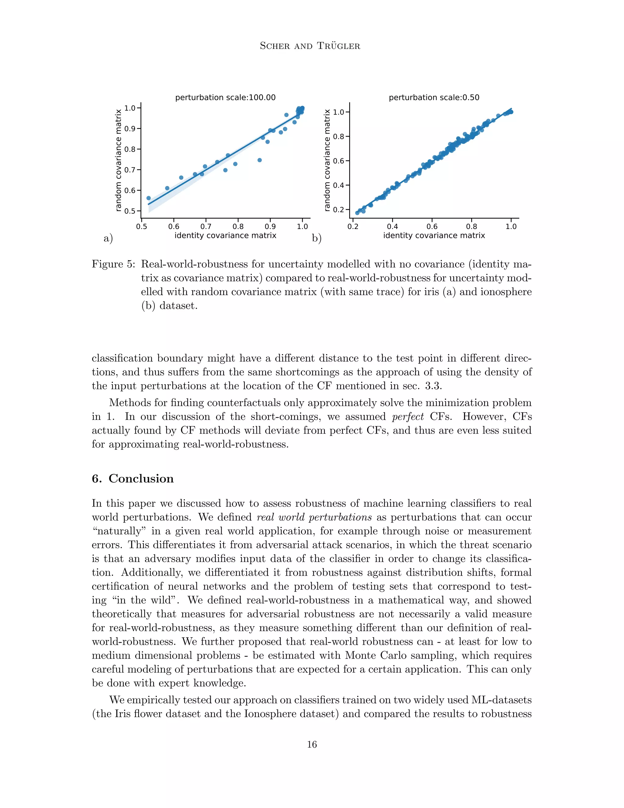
This document discusses assessing the robustness of machine learning models to "real-world perturbations" that occur naturally rather than being crafted by an adversary. It argues that adversarial robustness is not a valid measure of robustness to such natural perturbations. The document proposes a probabilistic approach to compute the likelihood that a real-world perturbation would change a model's prediction, quantifying its real-world robustness. This approach models possible input perturbations individually for each application and works for any "black-box" model. It illustrates the approach on two datasets and analytically solvable cases, and discusses estimating real-world robustness in high-dimensional spaces.

1. Robustness Beyond Adversarial Attacks
Robustness of Machine Learning Models Beyond Adversarial
Attacks
Sebastian Scher sscher@know-center.at
Know-Center GmbH
Inffeldgasse 13/6
8010 Graz, Austria
Andreas Trügler atruegler@know-center.at
Know-Center GmbH
Inffeldgasse 13/6
8010 Graz, Austria
and
Institute of Interactive Systems and Data Science
Graz University of Technology
Inffeldgasse 16C, 8010 Graz, Austria
and
Department of Geography and Regional Science
University of Graz
Heinrichstraße 36, 8010 Graz, Austria
Abstract
Correctly quantifying the robustness of machine learning models is a central aspect
in judging their suitability for specific tasks, and thus, ultimately, for generating trust in
the models. We show that the widely used concept of adversarial robustness and closely
related metrics based on counterfactuals are not necessarily valid metrics for determining
the robustness of ML models against perturbations that occur “naturally”, outside specific
adversarial attack scenarios. Additionally, we argue that generic robustness metrics in prin-
ciple are insufficient for determining real-world-robustness. Instead we propose a flexible
approach that models possible perturbations in input data individually for each application.
This is then combined with a probabilistic approach that computes the likelihood that a
real-world perturbation will change a prediction, thus giving quantitative information of
the robustness of the trained machine learning model. The method does not require access
to the internals of the classifier and thus in principle works for any black-box model. It
is, however, based on Monte-Carlo sampling and thus only suited for input spaces with
small dimensions. We illustrate our approach on two dataset, as well as on analytically
solvable cases. Finally, we discuss ideas on how real-world robustness could be computed
or estimated in high-dimensional input spaces.
Keywords: Robustness, Black Box Models, Trustworthy AI, Testing of AI, Reliability
1. Introduction
“Robustness” is a term widely used in the context of machine-learning (ML) and statistics.
In ML, it usually refers to how robust a model-prediction is to specific perturbations in the
1
arXiv:2204.10046v1
[cs.LG]
21
Apr
2022

2. Scher and Trügler
input data. A widely studied field is adversarial robustness, closely related to adversarial
examples (e.g. Szegedy et al., 2014; Goodfellow et al., 2015). Adversarial robustness (first
described in Szegedy et al. (2014) for neural networks) deals with the susceptibility of an
ML model to perturbations that were specifically crafted to “fool” the model - so called ad-
versarial attacks. Here the threat-model is that an attacker starts from a correctly classified
input (e.g. an image), and then modifies the input image with a minimal - often imper-
ceptible - perturbation that still leads to a misclassification. These perturbations typically
look random, but they are in fact not random and exploit specific characteristics of the ML
model and/or the training data.
While adversarial robustness is an important topic, it only deals with a certain type of
perturbations/attack-scenarios. In this paper, we deal with a different question: How can we
assess the robustness of a ML-model to perturbations that are not crafted by an adversarial
attacker, but that occur by chance and/or accident? We will call these perturbations
real-world-perturbations. Such perturbations could occur - among others - from: noise,
measurement errors, data-drift and data-processing errors. In this paper we will show that
adversarial robustness is not necessary a valid measure for the robustness against such
perturbations. Throughout this paper, the term real-world-perturbations will only refer to
this type of perturbations.
It is impossible to completely separate our idea of real-world-perturbations from other
central aspects in ML, namely generalization and distribution-shift. Additionally, the ques-
tion of how to acquire a suitable test-set is related, as well as the concept of counterfactuals
and the ideas behind data-augmentation (including test-time augmentation (Shanmugam
et al., 2020)).
1.1 Contributions
We start our discussion with a different angle of view compared to earlier works and focus
on the main question:
Given a trained ML application and a test-dataset, how can we assess the robustness to
perturbations that could occur when deploying the model in a real application, but are
not represented in the test set?
And more specifically:
How can we assess the robustness of a single test sample?
To answer these questions, in this paper we will
• define real-world-robustness in a mathematical way,
• argue why adversarial robustness and metrics based on counterfactuals are insufficient
for determining real-world-robustness,
• show how to compute real-world-robustness for low-dimensional datasets,
• compare adversarial robustness with real-world-robustness in two examples,
• discuss issues surrounding transferring the ideas to high-dimensional problems.
2

3. Robustness Beyond Adversarial Attacks
Another major difference compared to earlier work is that our approach is independent
(or in other words, completely ignorant) of the training data, and has thus to be differenti-
ated from all related concepts that have something to do with training data (e.g. robustness
to noise in training data). Our method starts from a trained classifier, where this classifier
comes from does not matter. It could even be a ”hand-coded” one (e.g. symbolic AI). Noise
tolerance in this sense is for example also an issue of lifelong learning machines (Kudithipudi
et al., 2022).
This work is addressed both to the research community and to practitioners in the grow-
ing field of testing and certifying AI-applications (Supreme Audit Institutions of Finland,
Germany, the Netherlands, Norway and the UK, 2020; Winter et al., 2021). Therefore, this
paper also aims to convey an intuitive understanding of the issues surrounding robustness
of ML models.
1.2 Taxonomy
We use the term robustness in the above described meaning. It should be noted that
sometimes robustness refers to how well a model works in other settings, and then the word
reliability is used instead to describe the sensitivity to small changes in the input (e.g. in
the NIST draft for a taxonomy of AI risk (NIST, 2021)).
2. Related Concepts and Related Work
In this section we discuss concepts that are related to our problem in the existing literature.
A recent review (Huang et al., 2020) also gives a broad overview on safety and trustworthi-
ness of deep neural networks with focus on related topics like verification, testing, adversarial
attack and defence, and interpretability.
2.1 Adversarial Examples, Counterfactuals and Adversarial Robustness
Adversarial examples are samples of input for a ML classification system that are very
similar to a normal input example, but cause the ML system to make a different classifi-
cation. A typical example are images that are slightly modified (often so slightly that the
difference is invisible by eye) and then lead to a misclassification. The concept is generic
and not limited to image recognition systems. Such adversarial examples exploit certain
properties of ML classifiers, and are explicitly and purposefully searched with specific al-
gorithms (called adversarial attacks). There is a lot of discussion in the literature on why
such examples do exist at all. In Szegedy et al. (2014) the authors suggested that adver-
sarial examples could be of extremely low probability. If this is true, then one would not
expect that they occur by chance (i.e. outside an adversarial attack scenario). Goodfellow
et al. (2015), however, disputed this low-probability explanation of adversarial examples,
and instead argued that they are caused by the local linearity of the neural networks. Other
perspectives/explanations have been offered as well (Ilyas et al., 2019; Tanay and Griffin,
2016). There is also literature on “real-world adversarial attacks” that deals with adver-
sarial attacks in real-world scenarios (Kurakin et al., 2017; Eykholt et al., 2018). This has,
however, nothing to do with our definition of real-world-robustness, as it still considers the
adversarial threat model.
3

4. Scher and Trügler
Counterfactuals (also known as counterfactual explanations (Kment, 2006)) are very
similar to adversarial examples. The idea is to find, for a given test data point, a different
data point with a different classification (either with a different classification of a specified
class, or with any classification different than the classification of the test point), under
the constraint that this example should be as similar as possible as the original test point.
It can thus be used for explaining classifications in a certain sense (“if feature x had a
value of b instead of a, then the classification would be different”). Such examples are
called counterfactuals. They have been first proposed in order to fullfill the “right to an
explanation” in the General Data Protection Regulation (GDPR) (Wachter et al., 2018;
Mittelstadt et al., 2019).
Adversarial examples and counterfactual explanations are highly related, up to the point
that they are sometimes seen as the same thing with two different names. Undisputed is that
both stem from the same mathematical optimization problem, and are thus mathematically
the same thing. Whether they are also semantically the same is part of ongoing discussions
as well. See Freiesleben (2021); Katz et al. (2017) for a thorough discussion on the topic.
Here, we do not attempt to answer that question, but instead use the terms interchangeably,
as for our setting the (potential) distinction is not important.
Usually, counterfactuals (and adversarial examples) require a pre-defined distance met-
ric. However, Pawelczyk et al. (2020) proposed a method that learns a suitable distance
metric from data. Many different methods for generating counterfactuals and adversarial
examples are known. Ten alone are integrated into the CARLA python library (Pawelczyk
et al., 2021), and additional ones in the Adversarial Robustness Toolbox (Nicolae et al.,
2019). Some methods work only on specific model types, others on black box models (like
CERTIFAI (Sharma et al., 2020))
In our paper, we discuss adversarial examples and counterfactuals agnostic of they way
they are be produced - we simply assume that they could somehow be obtained.
Together with the idea of adversarial attacks, the concept of measuring adversarial
robustness emerged. This is a measure to quantify how robust (or susceptible) a classifier
is to adversarial attacks. Two examples of ways to estimate adversarial robustness are the
CLEVER score, which is an attack-agnostic robustness metric for NNs (Weng et al., 2018),
and the CERTIFAI-robustness score for black box models, which assigns a robustness score
for individual data points based on the distance to the closest counterfactuals using a genetic
algorithm (Sharma et al., 2020).
2.2 Perturbation Theory and Interpretability Methods
If small perturbations are introduced to a physical system (e.g. noise, fluctuations, etc.)
it is often very helpful to develop a truncated power series expansion in terms of these
perturbations in order to find approximate solutions of the system. The perturbed system
can then be described as a simpler (ideally mathematical directly solvable) system plus cor-
responding correction terms, a very common approach in quantum mechanics for example.
The mathematical foundation behind is called perturbation theory and the general question
of how (small) perturbations are affecting a system of interest is obviously also linked to our
discussion here. While a direct assessment of a perturbation theoretic approach is beyond
the scope of our paper, at least related concepts have found their way to modern machine
4

5. Robustness Beyond Adversarial Attacks
learning literature as well. Investigating the influence of perturbations of input data (Olden
and Jackson, 2002) or analyzing machine model behaviour based on power series decom-
position (Montavon et al., 2017) have been introduced especially in the field of explainable
AI for example. One of the most popular methods to identify the influence of specific
input features in the output of a machine learning model (so-called attribution methods)
is based on perturbing the input. A description of CAPTUM, an open-source library for
interpretability methods containing generic implementations of a number of gradient and
perturbation-based attribution algorithms, as well as a set of evaluation metrics for these
algorithms, can be found in Kokhlikyan et al. (2020). Such approaches usually focus on
“faithfullness”, e.g. the ability of a machine learning algorithm to recognize important
features, instead of the overall robustness of the model.
2.3 Data Augmentation
Data augmentation are techniques to artificially create new training samples from existing
training data. It is widely used in tasks that work with images, as for image recognition it is
relatively easy to find modifications that change the image, but in a way that the image still
contains the same semantic information. Data augmentation is used to prevent overfitting.
Therefore, it is indirectly related to robustness, as the robustness of a classifier also depends
on its generalization properties, but it cannot be used as a measure for robustness. Data
augmentation is usually used during model training and not when the trained model is
evaluated. There is, however, also the idea of test-time data augmentation (Shanmugam
et al., 2020). Here “test-time” refers to making predictions with the model after training.
This is used because it can help improve the predictions, but it is also only indirectly related
to robustness.
2.4 Distribution Shift
Distribution shift (Federici et al., 2021; Bengio et al., 2019; Hendrycks et al., 2021) is the
phenomenon when the training data does not completely represent the test data that is
encountered in a real world application. A curated benchmark of various datasets reflecting
a diverse range of naturally occurring distribution shifts (such as shifts arising from different
cameras, hospitals, molecular scaffolds, experiments, demographics, countries, time periods,
users, and codebases) can be found in Koh et al. (2021). Robustness against distribution
shift (Taori et al., 2020) is closely related to the ability of a ML classifier to generalize to
points beyond the training examples and also to overfitting as a counterpart to generaliza-
tion.
Our definition of real-world robustness differs from distribution shifts, and it is not true
in a general sense that models that generalize well are automatically robust within our
real-world-robustness definition. Still, distribution shifts are also a relevant issue when
determining real-world-robustness in our approach. We model possible real world distribu-
tions, but when the application is put in practice, it might be that the actual occurring
perturbations are different - thus representing a distribution shift in the possible pertur-
bations. Yet another similar topic is robustness towards out-of-distribution points (Yang
et al., 2021), which focuses on unusual data that was not observed in the training dataset
(e.g. a self-driving cat that detects a new object type it has never seen before).
5

6. Scher and Trügler
2.5 Certification of Neural Networks
For neural networks (NNs) there is a lot of active research on finding formal guarantees and
thus “proofing” that a network is robust to particular perturbations and/or fulfills other
properties. This is often referred to as “verification” or “certification” (Singh et al., 2019).
For example, it is possible to find robustness guarantees for NNs with defining hypercubes
around test points, and then test whether the classification stays the same for all areas
within this hypercube. At the moment, this is only possible with strong assumptions and
restrictions on the possible perturbations (e.g. (Cohen et al., 2019; Singh et al., 2019)).
Huang et al. (2017) proposed a method that can offer high guarantees, but under the
restriction that input perturbations need to be discretized.
2.6 Robustness to Noise in Training Data
Sáez et al. (2016b) define robustness as “A robust classification algorithm can build models
from noisy data which are more similar to models built from clean data.” This robustness
against noise refers to the ability of the training algorithm to deal with noisy training data
(noise can be on the features and/or on the labels). The Relative Loss of Accuracy (RLA)
score proposed by Sáez et al. (2011) and the Equalized Loss of Accuracy (ELA) score
proposed by Sáez et al. (2016a) are ways of measuring this type of robustness (specifically
to noise on the class labels). This idea of robustness, however, is fundamentally different
from our definition of robustness, which deals with robustness of the trained classifier against
noise (and other perturbations) added to test samples. A systematic overview of the impact
of noise on classifiers is given in Zhu and Wu (2004), and the effect of label noise on the
complexity of classification problems in Garcia et al. (2015).
3. Methods
In this section we formalize our question on how to asses real-world-robustness, show why
adversarial samples and counterfactuals are insufficient for that purpose, and discuss how
to compute real-world robustness.
3.1 Adversarial Examples and Counterfactuals
Untargeted counterfactuals xc (or untargeted adversarial examples) with respect to a test
point x are defined via the following minimization problem (e.g. Freiesleben (2021)):
minimize d (xc, x) subject to f (xc) 6= f (x) , (1)
where d is a distance function that needs to be pre-defined and f is the corresponding
machine learning model.
There is also the concept of targeted counterfactuals or adversarial attacks, in which
the goal is not only that the counterfactual has a different predicted label, but a specific
different one. In this paper we only speak about untargeted counterfactuals and adversarial
examples. For binary classification problems (which will be used in this study as examples),
targeted and untargeted counterfactuals are per definition the same. Many different meth-
6

7. Robustness Beyond Adversarial Attacks
ods have been proposed to (approximately) solve this minimization problem (see references
in Introduction).
3.2 Real-world-robustness
Formally, our definition of real-world-robustness can be stated in the following way: given
a trained machine learning model f, a test-data point1 xt and the accompanying predicted
label y = f (xt), how can we assess how robust y is to perturbations x0 of xt? We consider
x0 not in an abstract way (e.g. a hypersphere), but as originating from real-world processes.
These can be, for example, noise or measurement errors.
We will use x0 for the perturbation, and x̂ for the perturbed value, thus
x̂ = xt + x0
.
Further, the perturbations x0 are not given in absolute values, but are described proba-
bilistically, leading to a N-dimensional probability density function p̂ (x0), which assigns a
probability density to each point x in the input space of the model. The input space has
dimension N, where N is the number of input features. Additionally, as in the real world we
cannot expect that potential perturbations are the same for all data-points, we introduce p̂
as a function dependent on xt
p̂(x0
) → p̂ xt, x0
.
Thus each test-point xt gets assigned a probability-distribution (defined over the input
space RN ).
To consider the example of measurements from temperature sensors, the noise of the
sensors might be different for high and for low temperatures. Or, another example, there
could be hard boundaries in some cases (e.g. a percentage range cannot be lower than 0 or
higher than 100).
The first challenge is thus to model p̂ (xt, x0). In principle there are two ways to model
p̂ (xt, x0): (1) analytically or (2) as a process that generates samples (e.g. via a Monte-Carlo
simulation). Both will require expert knowledge, and details of the specific application.
The second challenge is to find out whether our ML-model f yields different predictions
in the region of interest around xt. Here we intentionally use the vague term region of
interest, as defining this is one of the main problems, and the approach we choose is part
of what distinguishes this work from previous work. One possible ansatz is to define hard
boundaries for x0 (and subsequently for x̂), and then try to find out whether the prediction
for f is the same for the whole region defined in this way, yielding a binary measure (either
whole region yields same prediction, or not). This is one of the things that previous work
on certifying neural networks are aiming at (e.g. Singh et al. (2019).). This approach
would be, however, contrary to our idea of describing possible perturbations as probability
distributions. We thus formulate the problem the following way:
How likely is it that the model prediction changes under the assumed perturbations?
1. We omit a vector notation for simplicity, all variables with x in our discussion are typically vectors with
dimension of the input space of the machine-learning model f.
7

8. Scher and Trügler
In mathematical terms, we want to know the probability that f (p̂ (xt, x0)) returns a
prediction label different from f (xt). For this we can define a binary function that returns
one if the prediction is different than the one for the original data point, and zero otherwise:
f0
xt, x0
=
(
0 f (xt + x0) = f (xt)
1 f (xt + x0) 6= f (xt)
(2)
Then we can, in principle, integrate f0 (p̂ (xt + x0)) over the whole input space and thus
obtain the probability for a different prediction compared to the unperturbed data point:
P (f (x̂) 6= f (xt)) =
Z
RN
f0
xt, x0
dx0
. (3)
In order to define a robustness measure we can compute
Pr = 1 − P
This is what from now we will refer to as real-world-robustness.
An important thing to realize is that there are many possible ways that P could exceed
a certain value: there could be a region on the other side of the decision boundary (thus in
a region where the predicted label is different) that is small but has high probability, but
equally well there can be situations where the density of p̂ is relatively small on the other
side of the decision boundary, but that the region is actually large. In the first situation,
there are not many different possible points around xt that could cause a wrong prediction,
but those points are not very unlikely. In the second situation, the points that would cause
a wrong prediction are all relatively unlikely, but there are many of them, thus making the
probability of getting one of them in a real setting is actually equally high as in the first
situation. This is illustrated in fig. 1 for a binary classifier. For simplicity, we will show only
illustrations of classifiers with a single decision boundary - all the principles here also apply
to more complicated settings were the decision boundary consists of multiple unconnected
pieces.
3.3 Why Counterfactuals are not Enough
The above discussed principle - that there are many different situations that can lead
to the same probability of misclassification for a given uncertainty distribution around
the data point - shows something important, namely that the shortest distance to the
decision boundary alone is not enough for determining the robustness of a prediction. To
revisit fig. 1: The right data point is much closer to the decision boundary than the left
one, and still both have the same robustness in our sense. This insight leads us to the
first conclusion of this paper: The distance to the closest counterfactuals (or adversarial
examples), as for example suggested in Sharma et al. (2020), is not sufficient for determining
robustness to perturbations that could occur by chance in the real world. In fig. 1, the
closest counterfactual to the left data point would be much further away than the closest
counterfactual for the right data-point - thus suggesting a different robustness - but in fact
we have demonstrated above that both points have the same robustness. This stems from
the different shapes of the decision boundary in the vicinity of the two points. Another
8

9. Robustness Beyond Adversarial Attacks
y=a
y=b
decision boundary
x1
x2
integral=probability
of misclassification
same integrated
probability
Figure 1: Example of a binary classifier with two-dimensional feature space. Two data-
points (black dots) with uncertainty around them - here an elliptical distribution,
the ellipses are lines of equal likelyhood. The purple line is the decision boundary
of a binary classifier. The left point shows a situation where all possibilities of
a misclassification are not very likely (all in regions of the elliptical distribution
with low probability), but these regions summed together are in fact quite large,
thus the probability of misclassification is not that low (indicated by the green
area). In other words, one needs to get relatively far away from the original data
point to get a misclassification, but this can happen in many different directions.
The right data-point illustrates a different scenario: here only in a small range of
directions a misclassification is possible, but in those directions a misclassification
is happening in regions of high likelyhood.
9

10. Scher and Trügler
example is given in fig. 2a): Here we have two data points (for simplicity again with both
data points having the same uncertainty), and the distance to their closest counterfactuals
(indicated as yellow dots) is the same for both points. Therefore, the distance would indicate
that they have the same robustness. However, due to the different shapes of the decision
boundary, the left point actually is less robust than the right one. This is the case for all
types of classifier that have curved decision boundaries (thus all non-linear classifiers). For
completeness we point out that for linear classifiers (e.g. logistic regression), the distance
to the closest counterfactual does not suffer from the above mentioned problems (but the
issues discussed below are still relevant even for linear classifiers).
Another reason why the distance to the closest counterfactual is not enough is depicted
in fig. 2b). Here we have three data points, all with the same distance to the decision
boundary, and thus the same distance to the closest counterfactual (orange points). In
this example, also the shape of the decision boundary is very similar in the vicinity of
all three data points. However, the uncertainty of the data points is not the same. All
points have elliptical uncertainty distributions, but with different orientation with respect
to the decision boundary. Therefore, their robustness against real-world perturbations is
not the same - the leftmost point is more robust than the others. At a first thought, one
might be tempted to think that the latter problem might be solved the following way:
Given the density distribution p (xt), we could compute the density at the location of the
counterfactual and use this as a robustness measure. In the example in fig. 2b) this would
indeed yield the desired result: The leftmost point would be rated more robust then the two
other points. However, if we return to the example in fig. 2a), then this approach would
immediately fail: Here both points would be rated equally robust - as the counterfactuals
lie on the same probability lines - but indeed we had shown above that in terms of real-
world-robustness, the left point is less robust than the right one. The opposite would be the
case in the example in fig. 1: Here the density at the location of the closest counterfactual
would be higher for the right than for the left point - but indeed the real-world robustness
is the same for both points.
We can thus draw our first conclusion:
For determining robustness against real-world perturbations, counterfactuals/adversarial
examples are insufficient.
This does of course not mean that counterfactuals/adversarial examples are useless in
that respect - it only means that they do not cover the whole picture.
3.4 Analytical Solutions
For combinations of certain types of classifiers and assumed uncertainties it is possible to
find analytical solutions to Eq. (3). In the Appendix this is shown for two examples: 1) A
linear classifier and 2) a non-linear rule-based model, where for both the uncertainty of the
test-points is assumed to be a multivariate Gaussian distribution.
10

11. Robustness Beyond Adversarial Attacks
a)
same distance to closest
counterfactual
integral=probability
of misclassification
higher
probability lower
probability
y=b
y=a
x1
x2
decision boundary
b)
more robust
less
robust
less
robust
decision boundary
closest
counterfactuals
distance to counterfactuals
is the same for all three datapoints,
but their real robustness is
not the same
x1
x2
Figure 2: Illustrations showing why the distance to the closest counterfactual is an insuffi-
cient measure for real-world-robustness.
3.5 Assessing Real-World Robustness with MC Sampling
In this section we describe a brute-force approach based on Monte-Carlo sampling that
in principle can approximate the real-world robustness of any black box classifier, on a
test-point by test-point basis:
1. Build a function that returns discrete samples from p̂.
2. Draw N samples from that function.
3. Test the black box function f with the new data points, and compute the fraction
that leads to a different classification than the original data point.
For N → ∞ this method should converge to the exact solution of Eq. (4).
The challenge now lies in accurately describing the uncertainty p̂. This needs to be done
on an application-by-application basis and will require expert knowledge. Here we only
outline some basic approaches that could be taken, in order to help practitioners.
3.5.1 Continuous Features
For continuous features, if appropriate for the application, the easiest approach would be
to define p̂ as a multivariate normal distribution. For n features, this can be defined via a
covariance matrix of shape n × n. This can account for both uncorrelated and correlated
uncertainty of the individual features.
3.5.2 Categorical Features
For categorical features one can work with transition matrices that describe transition-
probabilities. If we have single categorical feature with m possible values this would result
in a (symmetric) m × m matrix. Each row (and each column) describes the transition
probability of one categorical value to all other categorical values.
11

12. Scher and Trügler
3.5.3 Regression Problems
The discussion in this paper focuses on classification problems - as does most of the literature
on robustness of machine learning algorithms. It is, however, possible to adapt our approach
to regression problems as well. In this case, Eq. (2) would need to be adjusted with a
threshold γ. If the difference between the regression output of the perturbed testpoint and
the original testpoint is smaller than the threshold, then the output is considered unchanged,
otherwise it is considered as changed:
f0
(xt, x) =
(
0 |f (x) − f (xt)| γ
1 |f (x) − f (xt)| γ
(4)
The rest remains the same as for classification problems.
3.6 Assessing Real-World-Robustness in High-Dimensional Datasets
The above described brute-force approach is bound to fail in settings with high-dimensional
feature spaces due to the curse of dimensionality. In order to explore the whole area of
interest around a test-point, a very huge number of samples would need to be drawn from
p̂, which is unfeasible. Finding solutions to (part) of this problem is actually the topic of all
work on certification and formal verification of neural networks mentioned in the introduc-
tion. However, to the best of our knowledge, no complete solution is known at the moment.
Instead, the literature focuses only on providing guarantees for certain aspects of input
perturbations. Work on adversarial robustness of course also deals with these issues and
partly provides solutions. However, as outlined in this paper, adversarial robustness is not
necessarily the same thing as robustness to real-world-perturbations. One interesting line
of research would be to rephrase the question behind formal guarantees of neural networks:
Instead of trying to find bounds within which perturbations do not change the prediction,
one could attempt to formally guarantee that the probability of misclassification under a
given (high-dimensional) perturbation strategy is below a certain probability threshold -
thus finding an upper bound for P in Eq. (3)
For certain applications, one could also use dimensionality-reduction to reduce the prob-
lem. The number of input features in the input space does not always have to the actual
dimensionality of the input data, as features can be (highly) correlated. It could be that in
some use-cases real-world-perturbations occur only - or a least mainly - along certain direc-
tions in feature space, which could coincide with the directions along which most variance
occurs in the training or test data. Methods for dimensionality reduction - such as Principal
Component Analysis (PCA) - could thus help in exploring the relevant space around test
points. This would be possible through modelling real-world-perturbations not on the full
input space, but on the leading principal components, or on feature found with stochastic
games Wicker et al. (2018). This will, however, never work generically. For example, in
some applications white noise will be a potential real world perturbation, but this will not
be represented at all in the leading principal components.
Other potential approaches:
12

13. Robustness Beyond Adversarial Attacks
• Try to use multiple different adversarial examples (e.g. not only the example closest
to the original point, but the n closest ones) as guidance towards the ”interesting”
direction(s) in feature space.
• For classifiers where the gradient of the output is available (e.g. for neural networks),
it would be possible to compare the direction of the largest absolute gradient at the
testpoint with the direction of highest probability in the assumed perturbation distri-
bution around the test point. If the two directions are similar, then the robustness is
lower. This could for example be based on the approach used in the CLEVER score
of Weng et al. (2018). Such an approach would be, however, closer to an extension of
adversarial robustness with information on perturbation distributions than a solution
for finding real-world-robustness in our definition.
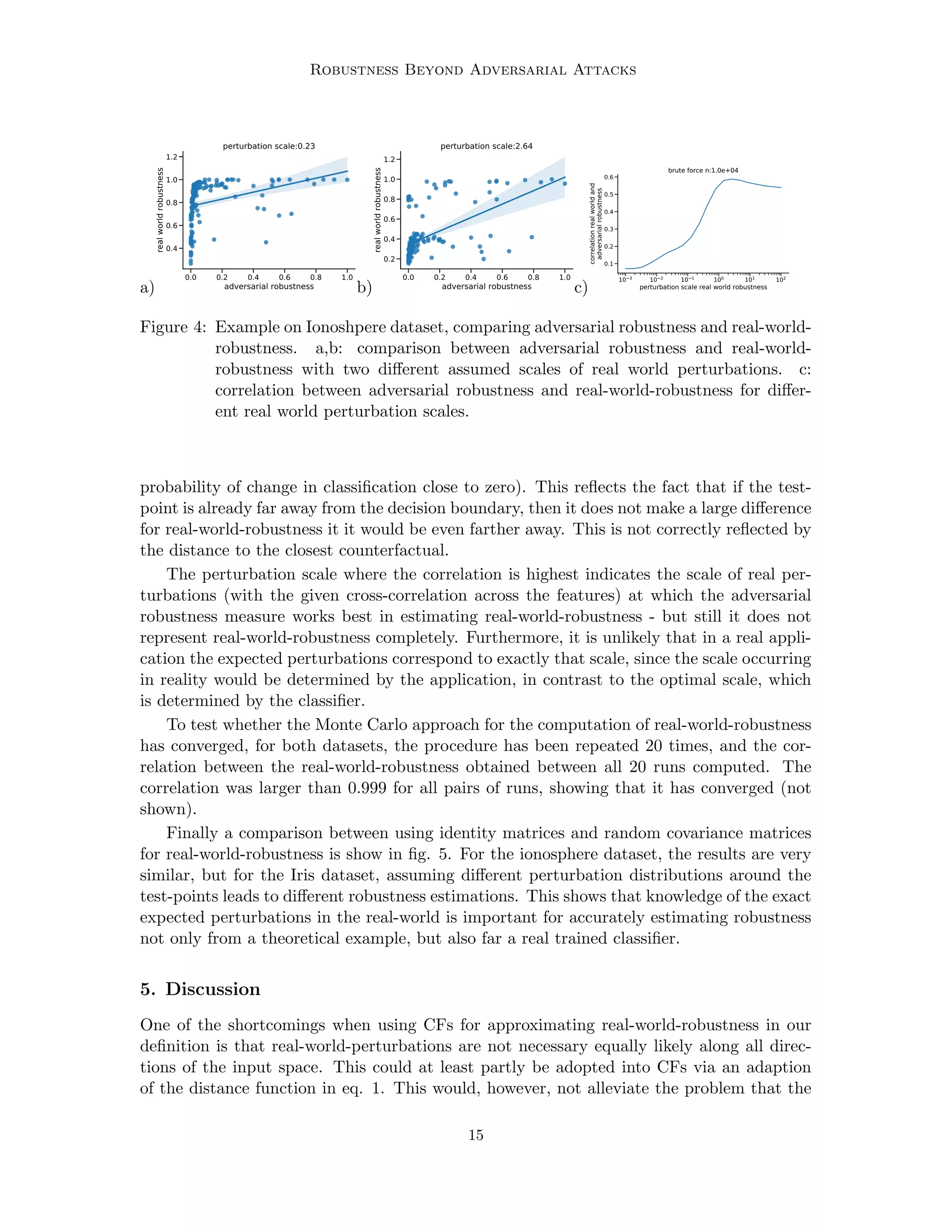
4. Examples
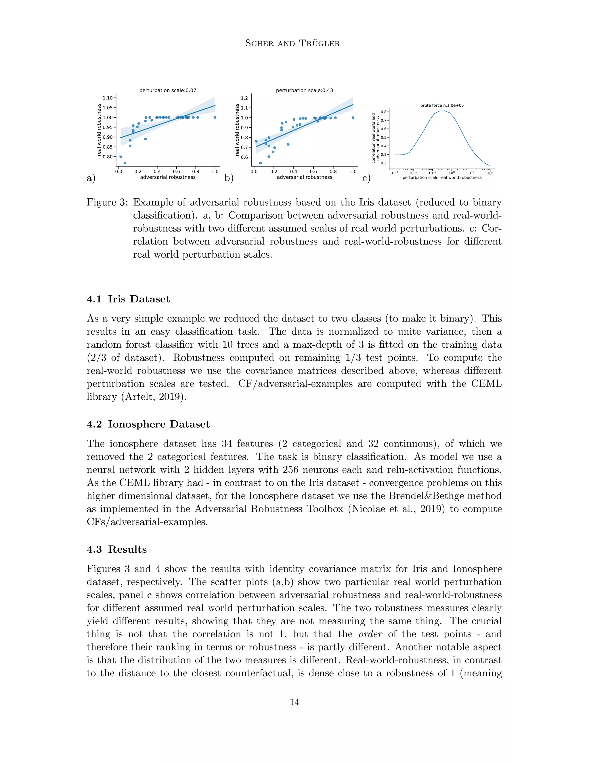
In this section we compare adversarial robustness with real-world robustness on classifiers
trained on two datasets: The Iris flower dataset (Anderson, 1936) and the Ionosphere
dataset (Sigillito et al., 1989), both available in the UCI repository (Dua and Graff, 2017).
The experiments we conduct are mainly for illustration purposes. On both datasets, a
classifier is trained, and then robustness is estimated with different assumptions on how
real-world perturbations could look like. We simply use two approaches as illustrations of
the concept, they do not necessarily correspond to what would be real-world perturbations
in applications that use classifiers based on these datasets.
For both datasets, we describe the expected uncertainty around the test-point as mul-
tivariate normal distributions, which are the same for each point (we thus assume that
the uncertainty of input features is independent of their value). The multivariate normal
distribution is described by a covariance matrix normalized to a trace of 1, and an overall
perturbation scale, which in our example is a scalar. We use two types of covariance matri-
ces, an identity matrix (no covariance terms, all diagonal terms 1) and random covariance
matrices (normalized to a trace of 1). The random covariance matrices are generated the
following way:
Cr = AT
A, (5)
where A is a matrix whose entries are all independently drawn from a normal distribution
with zero mean and unit variance. Eq. (5) ensures that Cr is a proper covariance matrix
(symmetric and positive semi-definite).
Real-world-robustness in our definition is a probability, and therefore contained in [0, 1].
The typical way of using adversarial examples as robustness measure is the distance di
between the test point xi and the closest adversarial example. This is a metric in (0, inf)
(in contrast to real-world-robustness, the distance cannot be zero, therefore the interval has
an open lower bound). In order to allow a better comparison, we rescale the distance to
the range (0, 1], thus we define adversarial robustness as
ri =
di
max (d1,2,.....N )
.
For each test point, N = 10000 samples from the perturbation distribution around the
test point are drawn for computing real-world-robustness.
13

14. Scher and Trügler
a)
0.0 0.2 0.4 0.6 0.8 1.0
adversarial robustness
0.80
0.85
0.90
0.95
1.00
1.05
1.10
real
world
robustness
perturbation scale:0.07
b)
0.0 0.2 0.4 0.6 0.8 1.0
adversarial robustness
0.6
0.7
0.8
0.9
1.0
1.1
1.2
real
world
robustness
perturbation scale:0.43
c)
10 3 10 2 10 1 100 101 102
perturbation scale real world robustness
0.2
0.3
0.4
0.5
0.6
0.7
0.8
correlation
real
world
and
adversarial
robustness
brute force n:1.0e+05
Figure 3: Example of adversarial robustness based on the Iris dataset (reduced to binary
classification). a, b: Comparison between adversarial robustness and real-world-
robustness with two different assumed scales of real world perturbations. c: Cor-
relation between adversarial robustness and real-world-robustness for different
real world perturbation scales.
4.1 Iris Dataset
As a very simple example we reduced the dataset to two classes (to make it binary). This
results in an easy classification task. The data is normalized to unite variance, then a
random forest classifier with 10 trees and a max-depth of 3 is fitted on the training data
(2/3 of dataset). Robustness computed on remaining 1/3 test points. To compute the
real-world robustness we use the covariance matrices described above, whereas different
perturbation scales are tested. CF/adversarial-examples are computed with the CEML
library (Artelt, 2019).
4.2 Ionosphere Dataset
The ionosphere dataset has 34 features (2 categorical and 32 continuous), of which we
removed the 2 categorical features. The task is binary classification. As model we use a
neural network with 2 hidden layers with 256 neurons each and relu-activation functions.
As the CEML library had - in contrast to on the Iris dataset - convergence problems on this
higher dimensional dataset, for the Ionosphere dataset we use the BrendelBethge method
as implemented in the Adversarial Robustness Toolbox (Nicolae et al., 2019) to compute
CFs/adversarial-examples.
4.3 Results
Figures 3 and 4 show the results with identity covariance matrix for Iris and Ionosphere
dataset, respectively. The scatter plots (a,b) show two particular real world perturbation
scales, panel c shows correlation between adversarial robustness and real-world-robustness
for different assumed real world perturbation scales. The two robustness measures clearly
yield different results, showing that they are not measuring the same thing. The crucial
thing is not that the correlation is not 1, but that the order of the test points - and
therefore their ranking in terms or robustness - is partly different. Another notable aspect
is that the distribution of the two measures is different. Real-world-robustness, in contrast
to the distance to the closest counterfactual, is dense close to a robustness of 1 (meaning
14

15. Robustness Beyond Adversarial Attacks
a)
0.0 0.2 0.4 0.6 0.8 1.0
adversarial robustness
0.4
0.6
0.8
1.0
1.2
real
world
robustness
perturbation scale:0.23
b)
0.0 0.2 0.4 0.6 0.8 1.0
adversarial robustness
0.2
0.4
0.6
0.8
1.0
1.2
real
world
robustness
perturbation scale:2.64
c)
10 3 10 2 10 1 100 101 102
perturbation scale real world robustness
0.1
0.2
0.3
0.4
0.5
0.6
correlation
real
world
and
adversarial
robustness
brute force n:1.0e+04
Figure 4: Example on Ionoshpere dataset, comparing adversarial robustness and real-world-
robustness. a,b: comparison between adversarial robustness and real-world-
robustness with two different assumed scales of real world perturbations. c:
correlation between adversarial robustness and real-world-robustness for differ-
ent real world perturbation scales.
probability of change in classification close to zero). This reflects the fact that if the test-
point is already far away from the decision boundary, then it does not make a large difference
for real-world-robustness it it would be even farther away. This is not correctly reflected by
the distance to the closest counterfactual.
The perturbation scale where the correlation is highest indicates the scale of real per-
turbations (with the given cross-correlation across the features) at which the adversarial
robustness measure works best in estimating real-world-robustness - but still it does not
represent real-world-robustness completely. Furthermore, it is unlikely that in a real appli-
cation the expected perturbations correspond to exactly that scale, since the scale occurring
in reality would be determined by the application, in contrast to the optimal scale, which
is determined by the classifier.
To test whether the Monte Carlo approach for the computation of real-world-robustness
has converged, for both datasets, the procedure has been repeated 20 times, and the cor-
relation between the real-world-robustness obtained between all 20 runs computed. The
correlation was larger than 0.999 for all pairs of runs, showing that it has converged (not
shown).
Finally a comparison between using identity matrices and random covariance matrices
for real-world-robustness is show in fig. 5. For the ionosphere dataset, the results are very
similar, but for the Iris dataset, assuming different perturbation distributions around the
test-points leads to different robustness estimations. This shows that knowledge of the exact
expected perturbations in the real-world is important for accurately estimating robustness
not only from a theoretical example, but also far a real trained classifier.
5. Discussion
One of the shortcomings when using CFs for approximating real-world-robustness in our
definition is that real-world-perturbations are not necessary equally likely along all direc-
tions of the input space. This could at least partly be adopted into CFs via an adaption
of the distance function in eq. 1. This would, however, not alleviate the problem that the
15

16. Scher and Trügler
a)
0.5 0.6 0.7 0.8 0.9 1.0
identity covariance matrix
0.5
0.6
0.7
0.8
0.9
1.0
random
covariance
matrix
perturbation scale:100.00
b)
0.2 0.4 0.6 0.8 1.0
identity covariance matrix
0.2
0.4
0.6
0.8
1.0
random
covariance
matrix
perturbation scale:0.50
Figure 5: Real-world-robustness for uncertainty modelled with no covariance (identity ma-
trix as covariance matrix) compared to real-world-robustness for uncertainty mod-
elled with random covariance matrix (with same trace) for iris (a) and ionosphere
(b) dataset.
classification boundary might have a different distance to the test point in different direc-
tions, and thus suffers from the same shortcomings as the approach of using the density of
the input perturbations at the location of the CF mentioned in sec. 3.3.
Methods for finding counterfactuals only approximately solve the minimization problem
in 1. In our discussion of the short-comings, we assumed perfect CFs. However, CFs
actually found by CF methods will deviate from perfect CFs, and thus are even less suited
for approximating real-world-robustness.
6. Conclusion
In this paper we discussed how to assess robustness of machine learning classifiers to real
world perturbations. We defined real world perturbations as perturbations that can occur
“naturally” in a given real world application, for example through noise or measurement
errors. This differentiates it from adversarial attack scenarios, in which the threat scenario
is that an adversary modifies input data of the classifier in order to change its classifica-
tion. Additionally, we differentiated it from robustness against distribution shifts, formal
certification of neural networks and the problem of testing sets that correspond to test-
ing “in the wild”. We defined real-world-robustness in a mathematical way, and showed
theoretically that measures for adversarial robustness are not necessarily a valid measure
for real-world-robustness, as they measure something different than our definition of real-
world-robustness. We further proposed that real-world robustness can - at least for low to
medium dimensional problems - be estimated with Monte Carlo sampling, which requires
careful modeling of perturbations that are expected for a certain application. This can only
be done with expert knowledge.
We empirically tested our approach on classifiers trained on two widely used ML-datasets
(the Iris flower dataset and the Ionosphere dataset) and compared the results to robustness
16

17. Robustness Beyond Adversarial Attacks
estimated with adversarial examples. The results were different, showing that the two
approaches do indeed measure two distinct things.
This shows that claims that robustness scores based on adversarial examples / counter-
factuals are generic robustness scores (such as in Sharma et al. (2020)) are not completely
true.
An inherent limitation in our proposed way for estimating real-world-robustness is that
it works only of the dimensionality of the input space is not too high. We discussed sev-
eral ideas on how this could be dealt with. For certain problems, it should be possible
to use dimensionality reduction techniques, but for general problems we cannot offer any
solution yet. We suspect that the research fields of adversarial robustness and formal guar-
antees for neural networks can provide valuable input to this point. Future research should
therefore, in addition to adversarial attack scenarios, also focus on how to determine real-
world-robustness for high-dimensional problems.
Finally, in this paper, we mainly dealt with black-box classifiers (except in the section
on analytical solutions). In cases where the classifier is known, and more specifically the
decision boundary(s) is known (such as in decision trees), it would also be possible to use
numerical integration to compute real-world-robustness (eq. 3). That would be done via
numerically integrating p over the region(s) where the classification is the same as for the
test point, and should in principle also work for high-dimensional datasets. This possibility
was not explored in this paper.
7. Code and Data Availability
The datasets we used are publicly available at the UCI repository https://archive.ics.
uci.edu/ml/index.php. All code developed for this study and links to the datasets are
available in the accompanying repository (repository will be published with the camera-
ready version of this paper).
Acknowledgments
We thank João de Freitas for interesting discussions.
This work was partly supported by the “DDAI” COMET Module within the COMET
– Competence Centers for Excellent Technologies Programme, funded by the Austrian Fed-
eral Ministry (BMK and BMDW), the Austrian Research Promotion Agency (FFG), the
province of Styria (SFG) and partners from industry and academia. The COMET Pro-
gramme is managed by FFG.
17

18. Scher and Trügler
Appendix A. Analytical solutions
The analytical solution of real-world-robustness is presented here for two simple cases: A
linear decision boundary, and a simple rule based model. Both are binary classifiers with
2-dimensional feature space.
A.1 Linear decision boundary
A linear decision boundary in 2-dimensional feature space can be described as
y (x1, x2) = w1x1 + w2x2 + b,
with the corresponding binary classifier function
f (x1, x2) =
(
0 y 1/2
1 y 1/2
For this classifier we can compute analytical solutions both for the distance to the closest
counterfactual as well as for our definition of real-world-robustness.
The closest counterfactual for a test-point (x1, x2) is obtained by minimizing the distance
from (x1, x2) to the decision boundary 1/2 = w1x1 +w2x2 +b. If we use euclidean distance,
this results in
xcf1 = −
2w2x2 + 2b + x1 − 1
2w1 − 1
xcf2 = −
2w1x1 + 2b + x2 − 1
2w2 − 1
The distance dcf to the counterfactual is given by
dcf =
q
(x1 − xcf1) + (x2 − xcf2).
We assume multivariate Gaussian uncertainty p (x1, x2, x0
1, x0
2) with covariance matrix
P
=
σ2
1 0
0 σ2
2
given by
p x1, x2, x0
1, x0
2
=
1
2σ1σ2
exp
−
(x0
1 − x1)2
2σ2
1
−
(x0
2 − x2)2
2σ2
2
#
. (6)
The real-world-robustness Pr, given by Eq. (3) in the main paper, can then be computed
as 1−P, where P is obtained by integrating p over the region of R2 where f (x + x0) 6= f (x).
Alternatively, Pr can be directly computed via p over the region of R2 where f (x + x0) =
f (x):
Pr (x1, x2) =
Z Z
f(x+x0)=f(x)
p x1, x2, x0
1, x0
2
dx0
2dx0
1. (7)
This equation can be solved via a rotation of the coordinate system such that one of the
rotated coordinate axes is parallel to the decision boundary.
18

19. Robustness Beyond Adversarial Attacks
4 3 2 1 0 1 2 3 4
x1
4
3
2
1
0
1
2
3
4
x
2 rwb
0.48
0.56
0.64
0.72
0.80
0.88
0.96
1.04
4 3 2 1 0 1 2 3 4
x1
4
3
2
1
0
1
2
3
4
x
2
distance to cf
0
2
4
6
8
10
12
14
Figure A.1: Analytical solution of real-world-robustness (left) and distance to closest coun-
terfactual (right) for a 2-dimensional linear decision boundary with w1 =
0, w2 = 1, b = 0 and Gaussian test-point uncertainty with σ = 1. Here the
distance to the closest counterfactual is not normalized.
For illustration purposes here we assume a classifier with w1 = 0 and b = 0, in which
case the decision boundary is parallel to the x1-axis.
In that case Eq. (7) simplifies to
Pr (x1, x2) =











∞
R
−∞
∞
R
1
2w2
p (x1, x2, x0
1, x0
2) dx0
2dx0
1 x2 1
2w2
∞
R
−∞
1
2w2
R
−∞
p (x1, x2, x0
1, x0
2) dx0
2dx0
1 x2 1
2w2
with the analytical solution
Pr (x1, x2) =



1
2 erf
2
√
2w2x2−
√
2
4 σ2w2
+ 1
2 x2 1
2w2
−1
2 erf
2
√
2w2x2−
√
2
4 σ2w2
+ 1
2 x2 1
2w2
(8)
where erf is the error function. Example plots for both robustness metrics are shown in
fig. A.1. Both are independent of x1, and decline steadily with larger distance along x2
from the decision boundary along. Distance to the closest counterfactual declines linear
with distance (per definition of the used distance metric), real-world-robustness declines
exponentially (because gaussian uncertaity is assumed).
A.2 Non-linear decision boundary
As an example of a non-linear classifier for which both robustness metrics can be analytically
computed we use the following decision function
19

20. Scher and Trügler
f (x1, x2) =
(
1 x1 a1 and x2 a2
0 else
which forms a decision boundary in 2d that looks like a right angle, where the tip of the
edge is at (a1, a2) . This could for example originate from a simple rule-based model, or a
decision tree with depth 2.
Distance to the closest counterfactual (i.e. distance to the decision boundary) is given
by
dcf (x1, x2) =

















min
q
(x1 − a1)2
,
q
(x2 − a2)2
x1 a1 and x2 a2
q
(x2 − a2)2
x1 a1 and x2 a2
q
(x1 − a1)2
x1 a1 and x2 a2
q
(x1 − a1)2
+ (x2 − a2)2
x1 a1 and x2 a2
The real-world-robustness thus follows as
Pr (x1, x2) =



























∞
Z
a2
∞
Z
a1
p x1, x2, x0
1, x0
2
dx0
1dx0
2 x1 a1 and x2 a2
∞
Z
−∞
a1
Z
−∞
p x1, x2, x0
1, x0
2
dx0
1dx0
2
+
a2
Z
−∞
∞
Z
a1
p x1, x2, x0
1, x0
2
dx0
1dx0
2
else
For uncertainty around the test points we use the same assumption as in the linear case
(Eq. 6). With this, Pr can be solved analytically again and yields
Pr (x1, x2) =

































1
4
erf
√
2x1 −
√
2
2 σ1
!
+ 1
!
erf
√
2x2 − 2
√
2
2 σ2
!
+
1
4
erf
√
2x1 −
√
2
2 σ1
!
+
1
4
x1 a1 and x2 a2
−
1
4
erf
√
2x1 −
√
2
2 σ1
!
+ 1
!
erf
√
2x2 − 2
√
2
2 σ2
!
−
1
4
erf
√
2x1 −
√
2
2 σ1
!
+
3
4
else
Example plots for both robustness metrics are shown in fig. A.2.
Far away from the corner the information of both metrics is similar. However, close the
the corner, they diverge. The distance to the closest counterfactual is only dependent on the
smallest distance (be it along x1 or x2). How much larger the distance along the other axis
20

21. Robustness Beyond Adversarial Attacks
2 1 0 1 2 3 4 5 6
x1
2
1
0
1
2
3
4
5
6
x
2 rwb
0.2
0.3
0.4
0.5
0.6
0.7
0.8
0.9
1.0
2 1 0 1 2 3 4 5 6
x1
2
1
0
1
2
3
4
5
6
x
2
distance to cf
0.0
0.8
1.6
2.4
3.2
4.0
4.8
5.6
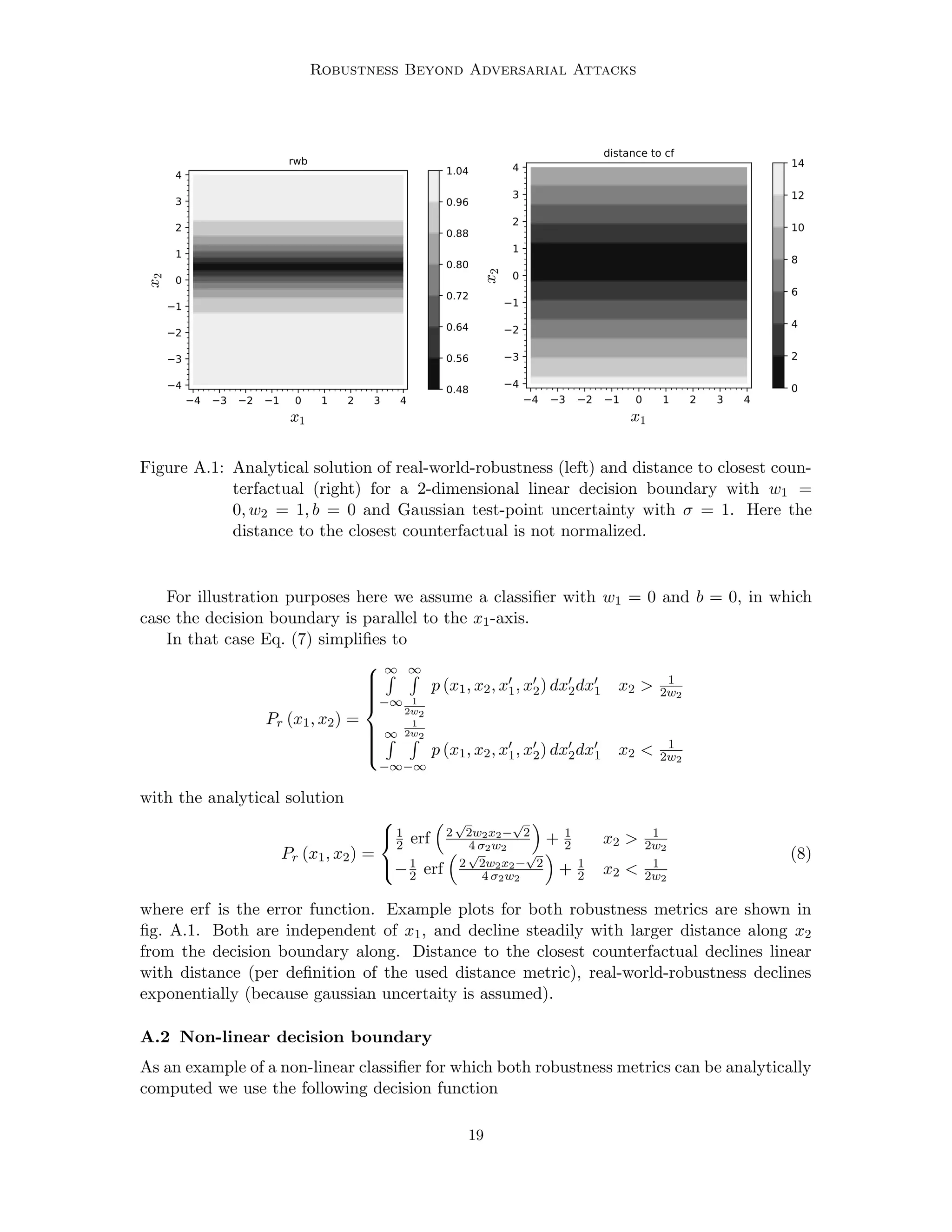
Figure A.2: Analytical solution of real-world-robustness (left) and distance to closest coun-
terfactuel (right) for a 2-dimensional linear decision boundary with w1 =
0, w2 = 1, b = 0 and Gaussian test-point uncertainty with σ = 1. Here the
distance to the closest counterfactual is not normalized.
is does not matter in this case. This is in contrast to our definition of real-world-robustness,
where it does matter: In close vicinity to the edges the decision boundary is close in both
directions, making the prediction less robust, as it can change from perturbations along both
axes. This is not correctly reflected when using the distance to the closest counterfactual
as robustness metric.
References
Edgar Anderson. The Species Problem in Iris. Annals of the Missouri Botanical Garden,
23(3):457, September 1936. ISSN 00266493. doi: 10.2307/2394164.
André Artelt. CEML: Counterfactuals for explaining machine learning models - a python
toolbox, 2019.
Yoshua Bengio, Tristan Deleu, Nasim Rahaman, Rosemary Ke, Sébastien Lachapelle, Olexa
Bilaniuk, Anirudh Goyal, and Christopher Pal. A meta-transfer objective for learning to
disentangle causal mechanisms, 2019.
Jeremy M. Cohen, Elan Rosenfeld, and J. Zico Kolter. Certified Adversarial Robustness
via Randomized Smoothing. arXiv:1902.02918 [cs, stat], June 2019.
Dheeru Dua and Casey Graff. UCI machine learning repository, 2017.
Kevin Eykholt, Ivan Evtimov, Earlence Fernandes, Bo Li, Amir Rahmati, Chaowei Xiao,
Atul Prakash, Tadayoshi Kohno, and Dawn Song. Robust Physical-World Attacks on
Deep Learning Models. arXiv:1707.08945 [cs], April 2018.
21

22. Scher and Trügler
Marco Federici, Ryota Tomioka, and Patrick Forré. An information-theoretic approach to
distribution shifts, 2021.
Timo Freiesleben. The Intriguing Relation Between Counterfactual Explanations and Ad-
versarial Examples. arXiv:2009.05487 [cs], August 2021.
Luı́s P. F. Garcia, André C. P. L. F. de Carvalho, and Ana C. Lorena. Effect of label noise
in the complexity of classification problems. Neurocomputing, 160:108–119, July 2015.
ISSN 0925-2312. doi: 10.1016/j.neucom.2014.10.085.
Ian J. Goodfellow, Jonathon Shlens, and Christian Szegedy. Explaining and Harnessing
Adversarial Examples. arXiv:1412.6572 [cs, stat], March 2015.
Dan Hendrycks, Steven Basart, Norman Mu, Saurav Kadavath, Frank Wang, Evan
Dorundo, Rahul Desai, Tyler Zhu, Samyak Parajuli, Mike Guo, Dawn Song, Jacob Stein-
hardt, and Justin Gilmer. The many faces of robustness: A critical analysis of out-of-
distribution generalization. In Proceedings of the IEEE/CVF International Conference
on Computer Vision (ICCV), pages 8340–8349, October 2021.
Xiaowei Huang, Marta Kwiatkowska, Sen Wang, and Min Wu. Safety verification of deep
neural networks. In International conference on computer aided verification, pages 3–29.
Springer, 2017.
Xiaowei Huang, Daniel Kroening, Wenjie Ruan, James Sharp, Youcheng Sun, Emese
Thamo, Min Wu, and Xinping Yi. A survey of safety and trustworthiness of deep neu-
ral networks: Verification, testing, adversarial attack and defence, and interpretability.
Computer Science Review, 37:100270, 2020. ISSN 1574-0137. doi: https://doi.org/10.
1016/j.cosrev.2020.100270. URL https://www.sciencedirect.com/science/article/
pii/S1574013719302527.
Andrew Ilyas, Shibani Santurkar, Dimitris Tsipras, Logan Engstrom, Brandon Tran, and
Aleksander Madry. Adversarial Examples Are Not Bugs, They Are Features. In Advances
in Neural Information Processing Systems, volume 32. Curran Associates, Inc., 2019.
Guy Katz, Clark Barrett, David Dill, Kyle Julian, and Mykel Kochenderfer. Reluplex: An
Efficient SMT Solver for Verifying Deep Neural Networks. arXiv:1702.01135 [cs], May
2017.
Boris Kment. Counterfactuals and explanation. Mind, 115(458):261–310, 2006. doi: 10.
1093/mind/fzl261.
Pang Wei Koh, Shiori Sagawa, Henrik Marklund, Sang Michael Xie, Marvin Zhang, Akshay
Balsubramani, Weihua Hu, Michihiro Yasunaga, Richard Lanas Phillips, Irena Gao, Tony
Lee, Etienne David, Ian Stavness, Wei Guo, Berton Earnshaw, Imran Haque, Sara M
Beery, Jure Leskovec, Anshul Kundaje, Emma Pierson, Sergey Levine, Chelsea Finn, and
Percy Liang. Wilds: A benchmark of in-the-wild distribution shifts. In Marina Meila
and Tong Zhang, editors, Proceedings of the 38th International Conference on Machine
Learning, volume 139 of Proceedings of Machine Learning Research, pages 5637–5664.
PMLR, 18–24 Jul 2021. URL https://proceedings.mlr.press/v139/koh21a.html.
22

23. Robustness Beyond Adversarial Attacks
Narine Kokhlikyan, Vivek Miglani, Miguel Martin, Edward Wang, Bilal Alsallakh, Jonathan
Reynolds, Alexander Melnikov, Natalia Kliushkina, Carlos Araya, Siqi Yan, and Orion
Reblitz-Richardson. Captum: A unified and generic model interpretability library for
pytorch, 2020.
Dhireesha Kudithipudi, Mario Aguilar-Simon, Jonathan Babb, Maxim Bazhenov, Douglas
Blackiston, Josh Bongard, Andrew P. Brna, Suraj Chakravarthi Raja, Nick Cheney, Jeff
Clune, Anurag Daram, Stefano Fusi, Peter Helfer, Leslie Kay, Nicholas Ketz, Zsolt Kira,
Soheil Kolouri, Jeffrey L. Krichmar, Sam Kriegman, Michael Levin, Sandeep Madireddy,
Santosh Manicka, Ali Marjaninejad, Bruce McNaughton, Risto Miikkulainen, Zaneta
Navratilova, Tej Pandit, Alice Parker, Praveen K. Pilly, Sebastian Risi, Terrence J. Se-
jnowski, Andrea Soltoggio, Nicholas Soures, Andreas S. Tolias, Darı́o Urbina-Meléndez,
Francisco J. Valero-Cuevas, Gido M. van de Ven, Joshua T. Vogelstein, Felix Wang, Ron
Weiss, Angel Yanguas-Gil, Xinyun Zou, and Hava Siegelmann. Biological underpinnings
for lifelong learning machines. Nature Machine Intelligence, 4(3):196–210, mar 2022. doi:
10.1038/s42256-022-00452-0.
Alexey Kurakin, Ian Goodfellow, and Samy Bengio. Adversarial examples in the physical
world. arXiv:1607.02533 [cs, stat], February 2017.
Brent Mittelstadt, Chris Russell, and Sandra Wachter. Explaining explanations in ai.
In Proceedings of the Conference on Fairness, Accountability, and Transparency, FAT*
’19, page 279–288, New York, NY, USA, 2019. Association for Computing Machinery.
ISBN 9781450361255. doi: 10.1145/3287560.3287574. URL https://doi.org/10.1145/
3287560.3287574.
Grégoire Montavon, Sebastian Lapuschkin, Alexander Binder, Wojciech Samek, and Klaus-
Robert Müller. Explaining nonlinear classification decisions with deep taylor decompo-
sition. Pattern Recognition, 65:211–222, 2017. ISSN 0031-3203. doi: https://doi.org/10.
1016/j.patcog.2016.11.008. URL https://www.sciencedirect.com/science/article/
pii/S0031320316303582.
Maria-Irina Nicolae, Mathieu Sinn, Minh Ngoc Tran, Beat Buesser, Ambrish Rawat, Martin
Wistuba, Valentina Zantedeschi, Nathalie Baracaldo, Bryant Chen, Heiko Ludwig, Ian M.
Molloy, and Ben Edwards. Adversarial Robustness Toolbox v1.0.0. arXiv:1807.01069 [cs,
stat], November 2019.
NIST. Draft - Taxonomy of AI Risk. page 9, 2021.
Julian D Olden and Donald A Jackson. Illuminating the “black box”: a randomization
approach for understanding variable contributions in artificial neural networks. Ecological
modelling, 154(1-2):135–150, 2002.
Martin Pawelczyk, Johannes Haug, Klaus Broelemann, and Gjergji Kasneci. Learning
Model-Agnostic Counterfactual Explanations for Tabular Data. Proceedings of The Web
Conference 2020, pages 3126–3132, April 2020. doi: 10.1145/3366423.3380087.
23

24. Scher and Trügler
Martin Pawelczyk, Sascha Bielawski, Johannes van den Heuvel, Tobias Richter, and Gjergji
Kasneci. CARLA: A Python Library to Benchmark Algorithmic Recourse and Counter-
factual Explanation Algorithms. arXiv:2108.00783 [cs], August 2021.
José A Sáez, Julián Luengo, and Francisco Herrera. Evaluating the classifier behavior
with noisy data considering performance and robustness: The equalized loss of accuracy
measure. Neurocomputing, 176:26–35, 2016a.
José A. Sáez, Julián Luengo, and Francisco Herrera. Evaluating the classifier behavior with
noisy data considering performance and robustness: The Equalized Loss of Accuracy
measure. Neurocomputing, 176:26–35, February 2016b. ISSN 0925-2312. doi: 10.1016/j.
neucom.2014.11.086.
Divya Shanmugam, Davis Blalock, Guha Balakrishnan, and John Guttag. When and Why
Test-Time Augmentation Works. arXiv:2011.11156 [cs], November 2020.
Shubham Sharma, Jette Henderson, and Joydeep Ghosh. CERTIFAI: A Common Frame-
work to Provide Explanations and Analyse the Fairness and Robustness of Black-box
Models. In Proceedings of the AAAI/ACM Conference on AI, Ethics, and Society, pages
166–172, New York NY USA, February 2020. ACM. ISBN 978-1-4503-7110-0. doi:
10.1145/3375627.3375812.
Vincent G Sigillito, Simon P Wing, Larrie V Hutton, and Kile B Baker. Classification of
radar returns from the ionosphere using neural networks. Johns Hopkins APL Technical
Digest, 10(3):262–266, 1989.
Gagandeep Singh, Timon Gehr, Markus Püschel, and Martin Vechev. An abstract domain
for certifying neural networks. Proceedings of the ACM on Programming Languages, 3
(POPL):1–30, January 2019. ISSN 2475-1421. doi: 10.1145/3290354.
Supreme Audit Institutions of Finland, Germany, the Netherlands, Norway and the UK.
Auditing machine learning algorithms - A white paper for public auditors. Technical
report, 2020.
Christian Szegedy, Wojciech Zaremba, Ilya Sutskever, Joan Bruna, Dumitru Erhan, Ian
Goodfellow, and Rob Fergus. Intriguing properties of neural networks. arXiv:1312.6199
[cs], February 2014.
José A. Sáez, Julián Luengo, and Francisco Herrera. Fuzzy rule based classification systems
versus crisp robust learners trained in presence of class noise’s effects: A case of study.
In 2011 11th International Conference on Intelligent Systems Design and Applications,
pages 1229–1234, 2011. doi: 10.1109/ISDA.2011.6121827.
Thomas Tanay and Lewis Griffin. A Boundary Tilting Persepective on the Phenomenon of
Adversarial Examples. arXiv:1608.07690 [cs, stat], August 2016.
Rohan Taori, Achal Dave, Vaishaal Shankar, Nicholas Carlini, Benjamin Recht, and Lud-
wig Schmidt. Measuring robustness to natural distribution shifts in image classifica-
tion. In H. Larochelle, M. Ranzato, R. Hadsell, M. F. Balcan, and H. Lin, editors,
24

25. Robustness Beyond Adversarial Attacks
Advances in Neural Information Processing Systems, volume 33, pages 18583–18599. Cur-
ran Associates, Inc., 2020. URL https://proceedings.neurips.cc/paper/2020/file/
d8330f857a17c53d217014ee776bfd50-Paper.pdf.
Sandra Wachter, Brent Mittelstadt, and Chris Russell. Counterfactual Explanations with-
out Opening the Black Box: Automated Decisions and the GDPR. arXiv:1711.00399
[cs], March 2018.
Tsui-Wei Weng, Huan Zhang, Pin-Yu Chen, Jinfeng Yi, Dong Su, Yupeng Gao, Cho-Jui
Hsieh, and Luca Daniel. Evaluating the Robustness of Neural Networks: An Extreme
Value Theory Approach. arXiv:1801.10578 [cs, stat], January 2018.
Matthew Wicker, Xiaowei Huang, and Marta Kwiatkowska. Feature-Guided Black-Box
Safety Testing of Deep Neural Networks. arXiv:1710.07859 [cs], February 2018.
Philip Matthias Winter, Sebastian Eder, Johannes Weissenböck, Christoph Schwald,
Thomas Doms, Tom Vogt, Sepp Hochreiter, and Bernhard Nessler. Trusted Artificial
Intelligence: Towards Certification of Machine Learning Applications. arXiv:2103.16910
[cs, stat], March 2021.
Jingkang Yang, Kaiyang Zhou, Yixuan Li, and Ziwei Liu. Generalized out-of-distribution
detection: A survey, 2021.
Xingquan Zhu and Xindong Wu. Class noise vs. attribute noise: A quantitative study.
Artificial intelligence review, 22(3):177–210, 2004.
25