Download to read offline


![2
2. Panel vector autoregression
We consider a -variate panel VAR of order with panel-specific fixed effects represented by the
following system of linear equations:
= + + ⋯ + + + + +
∈ {1,2, … , }, ∈ {1,2, … , }
(1)
where is a (1 ) vector of dependent variables; is a (1 ) vector of exogenous covariates;
and are (1 ) vectors of dependent variable-specific fixed-effects and idiosyncratic errors,
respectively. The ( ) matrices , , … , , and the ( ) matrix are parameters to be
estimated. We assume that the innovations have the following characteristics: [ ] = , [ ] =
and [ ] = for all > .
The parameters above may be estimated jointly with the fixed effects or, alternatively, independently of
the fixed effects after some transformation, using equation-by-equation ordinary least squares (OLS).
With the presence of lagged dependent variables in the right-hand side of the system of equations,
however, estimates would be biased even with large (Nickell, 1981). Although the bias approaches
zero as gets larger, simulations by Judson and Owen (1999) find significant bias even when = 30.
2.1.GMM estimation
Various estimators based on GMM have been proposed to calculate consistent estimates of the above
equation, especially in fixed and large settings.4
With our assumption that errors are serially
uncorrelated, the first-difference transformation may be consistently estimated equation-by-equation
4
Other methods include analytical bias correction for the least squares dummy variable model, e.g. Kiviet (1995),
and Bun and Carree (2005), bias correction based on bootstrap methods, e.g. Everaert and Pozzi (2007), among
others. See Canova and Ciccarelli (2013) for a survey of panel VAR models.](https://image.slidesharecdn.com/abrigoandlove2015-171202104944/75/Abrigo-and-love_2015_-3-2048.jpg)
![4
∗
= ∗ ∗
… ∗ ∗
∗
= [ ∗ ∗
… ∗ ∗ ∗
]
∗
= ∗ ∗
… ∗ ∗
′ = ′ ′ … ′ ′
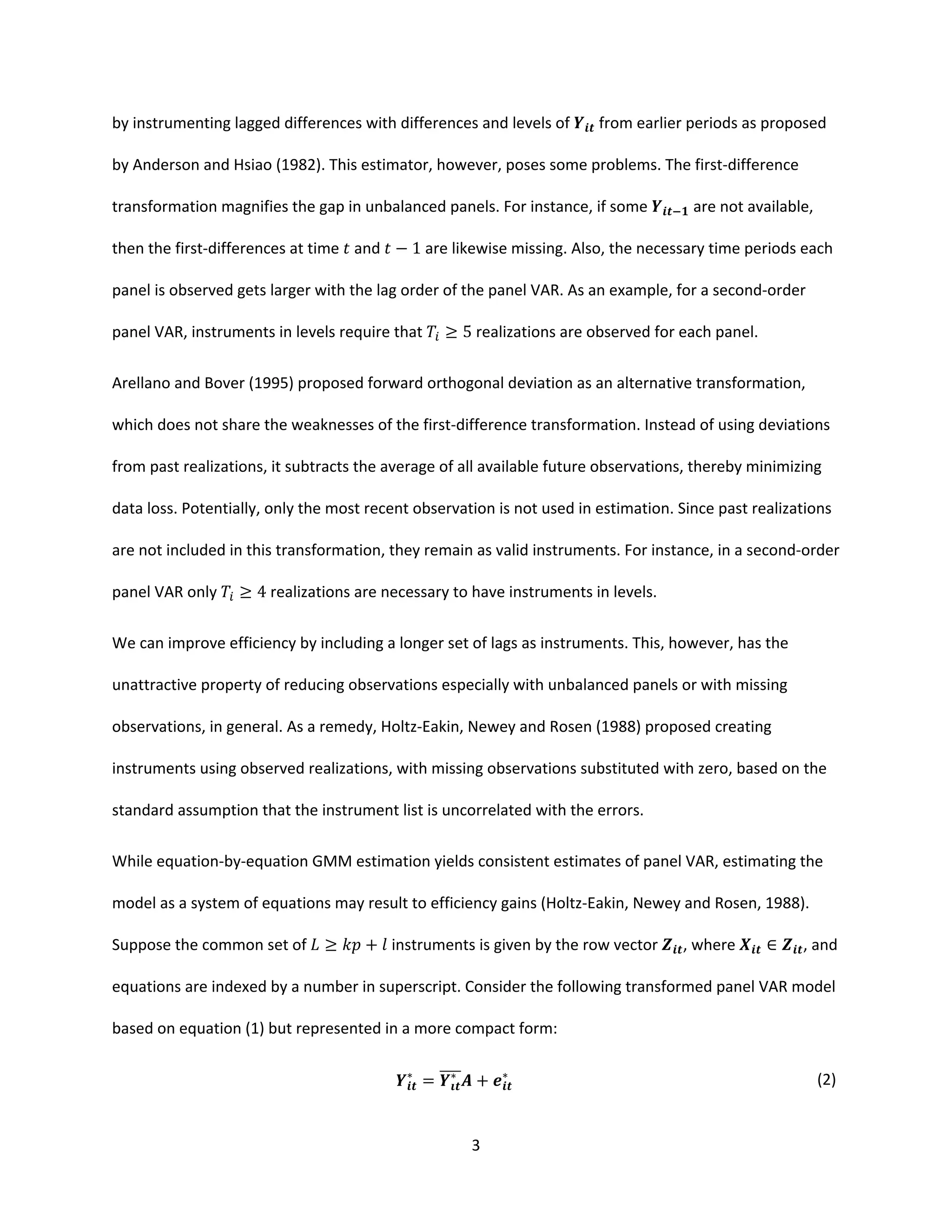
where the asterisk denotes some transformation of the original variable. If we denote the original
variable as , then the first difference transformation imply that ∗
= − , while for the
forward orthogonal deviation = ( − ) /( + 1) , where is the number of available
future observations for panel at time , and is its average.
Suppose we stack observations over panels then over time. The GMM estimator is given by
= ∗′ ′ ∗ ( ∗′ ′ ∗
) (3)
where is a ( ) weighting matrix assumed to be non-singular, symmetric and positive semi-
definite. Assuming that [ ] = and rank ∗ = + , the GMM estimator is consistent. The
weighting matrix may be selected to maximize efficiency (Hansen, 1982).5
Joint estimation of the system of equations makes cross-equation hypothesis testing straightforward.
Wald tests about the parameters may be implemented based on the GMM estimate of and its
covariance matrix. Granger causality tests, with the hypothesis that all coefficients on the lag of variable
are jointly zero in the equation for variable , may likewise be carried out using this test.
5
Roodman (2009) provides an excellent discussion of GMM estimation in a dynamic panel setting and its
applications using Stata. Readers are encouraged to read his paper for a more detailed discussion of this topic.](https://image.slidesharecdn.com/abrigoandlove2015-171202104944/75/Abrigo-and-love_2015_-5-2048.jpg)


![7
Impulse-response function confidence intervals may be derived analytically based on the asymptotic
distribution of the panel VAR parameters and the cross-equation error variance-covariance matrix.
Alternatively, the confidence interval may likewise be estimated using Monte Carlo simulation, and
bootstrap resampling methods.6
2.4.Forecast-error variance decomposition
The ℎ-step ahead forecast-error can be expressed as
− [ ] = ( ) (10)
where is the observed vector at time + ℎ and [ ] is the ℎ-step ahead predicted vector
made at time . Similar to impulse-response functions, we orthogonalize the shocks using the matrix
to isolate each variable’s contribution to the forecast-error variance. The orthogonalized shocks
have a covariance matrix , which allows straightforward decomposition of the forecast-error variance.
More specifically, the contribution of a variable to the ℎ-step ahead forecast-error variance of
variable may be calculated as
= ( ) (11)
where is the -th column of . In application, the contributions are often normalized relative to the
ℎ-step ahead forecast-error variance of variable
. = ′ (12)
6
See for instance Lutkepohl (2005) for details applied in time-series VAR.](https://image.slidesharecdn.com/abrigoandlove2015-171202104944/75/Abrigo-and-love_2015_-8-2048.jpg)
![8
Similar to impulse-response functions, confidence intervals may be derived analytically or estimated
using various resampling techniques.
3. Stata syntax
Model selection, estimation and inference about the panel vector autoregression model above can be
implemented with the new Stata commands pvar, pvarsoc, pvargranger, pvarstable, pvarirf
and pvarfevd. The syntax and outputs are closely patterned after Stata’s built-in var commands for
ease of use in switching between panel and time series VAR. We describe the commands’ syntax in this
section and provide examples in section 4.
3.1.pvar
pvar estimates panel vector autoregression models by fitting a multivariate panel regression of each
dependent variable on lags of itself, lags of all other dependent variables and exogenous variables, if
any. The estimation is by generalized method of moments (GMM). The command is implemented using
the interactive version of Stata’s gmm with analytic derivatives.
Syntax
pvar depvarlist [if] [in] [, options]
Options
lags(#) specifies the maximum lag order # to be included in the model. The default is to use the first
lag of each variable in depvarlist.
exog(varlist) specifies a list of exogenous variables to be included in the panel VAR.](https://image.slidesharecdn.com/abrigoandlove2015-171202104944/75/Abrigo-and-love_2015_-9-2048.jpg)
![9
fod and fd specifies how the panel-specific fixed effects will be removed. fod specifies that the panel
fixed-effects be removed using forward orthogonal deviation or Helmert transformation. By
default, the first # lags of transformed depvarlist in the model are instrumented by the same
lags in level (i.e. untranformed). fod is the default option. fd specifies that the panel-specific
fixed effects be removed using first difference instead of forward orthogonal deviations. By
default, the first # lags of transformed (i.e. differenced) depvarlist in the model are
instrumented by the #+1 to 2#+1 lags of depvarlist in levels (i.e. untransformed).
td subtracts from each variable in the model its cross-sectional mean before estimation. This could be
used to removed time fixed effects from all the variables prior to any other transformation.
instlags(numlist) overrides the default lag orders of depvarlist used as instruments in the
model (see fod and fd options above which describe which lags are used as default). Instead the
numlist-th lags are used as instruments.
gmmstyle specifies that "GMM-style" instruments as proposed by Holtz-Eakin, Newey and Rosen
(1988) be used. For each instrument based on lags of depvarlist, missing values are substituted
with zero. Observations with no valid instruments are excluded. This option is available only with
instlags().
gmmopts(options) overrides the default gmm options run by pvar. Each equation in the model may
be accessed individually using the variable names in depvarlist as equation names.
vce(vcetype[, independent]) specifies the type of standard error reported, which includes types
that are robust to some types of misspecification, that allow for intragroup correlation, and that
use bootstrap or jackknife methods.
overid specifies that Hansen's J statistic of over-identifying restriction be reported. This option is
available only for over-identified systems.](https://image.slidesharecdn.com/abrigoandlove2015-171202104944/75/Abrigo-and-love_2015_-10-2048.jpg)

![12
of the least restrictive panel VAR model, i.e. with the highest lag order used, for all models that would
be estimated by the program.
Syntax
pvarsoc depvarlist [if] [in] [, options]
Options
maxlag(#) specifies the maximum lag order for which the statistics are obtained.
pinstlag(numlist) specifies that the numlist-th lag from the highest lag order of depvarlist
specified in the panel VAR model implemented using pvar be used. This option cannot be
specified with the option pvaropts(instlag(numlist)).
pvaropts(options) passes arguments to pvar. All arguments specified in options are passed to
and used by pvar in estimation.
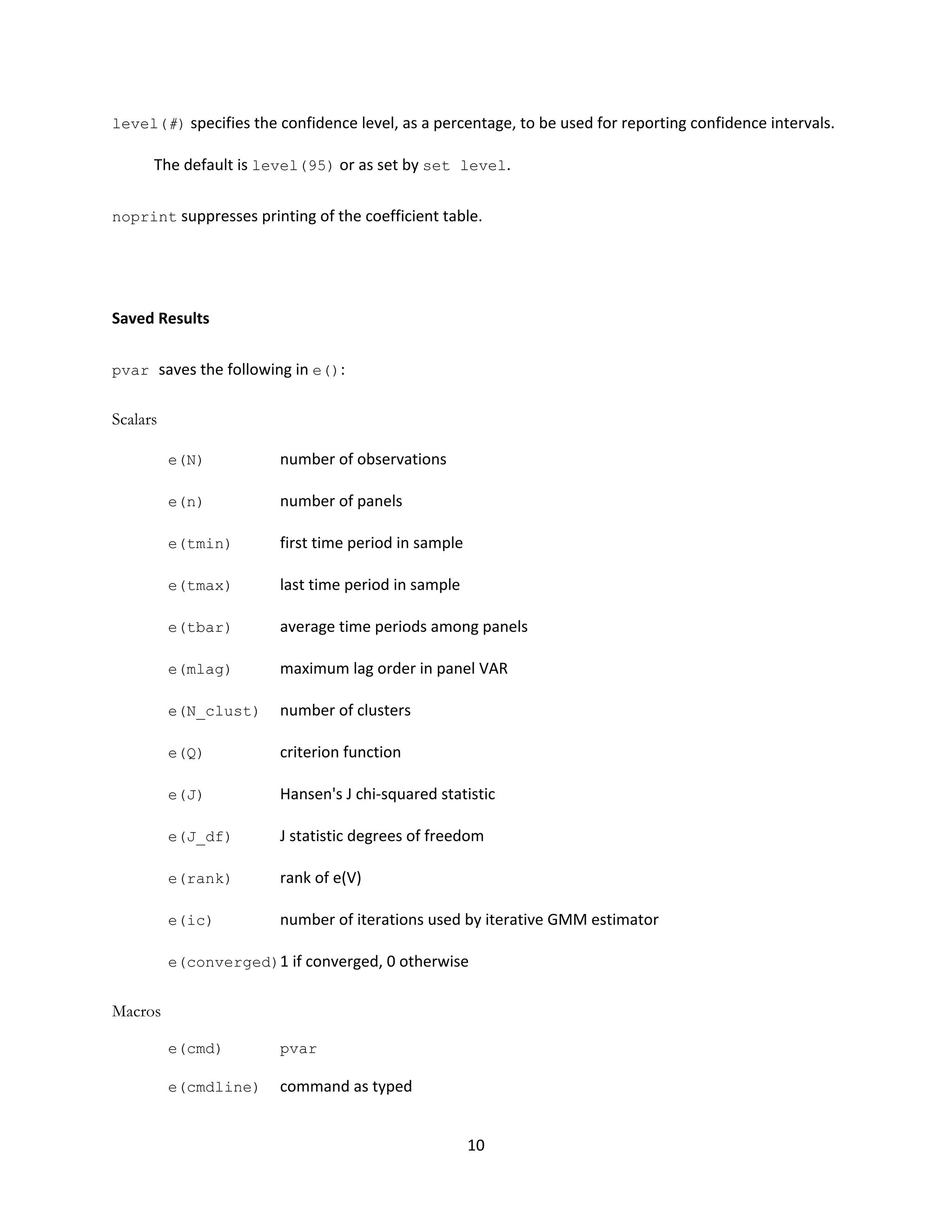
Saved Results
pvarsoc saves the following in r():
Scalars
r(N) number of observations
r(n) number of panels
r(tmin) first time period in sample
r(tmax) last time period in sample
r(tbar) average time periods among panels
r(maxlag) maximum lag order in panel VAR
Macros
r(endog) names of endogenous variables](https://image.slidesharecdn.com/abrigoandlove2015-171202104944/75/Abrigo-and-love_2015_-13-2048.jpg)
![13
r(exog) names of exogenous variables, if specified
Matrices
r(stats) CD, J and p-value, MBIC, MAIC, and MQIC
3.3.pvargranger
The post-estimation command pvargranger performs Granger causality Wald tests for each equation
of the underlying panel VAR model. It provides a convenient alternative to Stata’s built-in test
command.
Syntax
pvargranger [, estimates(estname)]
Options
estimates(estname) requests that pvargranger use the previously obtained set of panel VAR
estimates saved as estname. By default, pvargranger uses the active (i.e. the latest) results.
Saved Results
pvargranger saves the following in r():
Matrix
r(pgstats) chi-squared, degrees of freedom, and p-values
3.4.pvarstable
The post-estimation command pvarstable checks the stability condition of panel VAR estimates by
calculating the modulus of each eigenvalue of the estimated model. Lutkepohl (2005) and Hamilton
(1994) both show that a VAR model is stable if all moduli of the companion matrix are strictly less than
one. Stability implies that the panel VAR is invertible and has an infinite-order vector moving-average](https://image.slidesharecdn.com/abrigoandlove2015-171202104944/75/Abrigo-and-love_2015_-14-2048.jpg)
![14
representation, providing known interpretation to estimated impulse-response functions and forecast-
error variance decompositions.
Syntax
pvarstable [, options]
Options
estimates(estname) requests that pvarstable use the previously obtained set of pvar estimates
saved in estname. By default, pvarstable uses the active estimation results.
graph requests pvarstable to draw a graph of the eigenvalue of the companion matrix.
nogrid suppresses the polar grid circles on the plotted eigenvalues.
Saved Results
pvarstable saves the following in r():
Matrices
r(Re) real part of the eigenvalues of the companion matrix
r(Im) imaginary part of the eigenvalues of the companion matrix
r(Modulus) modulus of the eigenvalues of the companion matrix
3.5.pvarirf
The post-estimation command pvarirf calculates and plots impulse-response functions (IRF).
Confidence bands are estimated using Gaussian approximation based on Monte Carlo draws from the
estimated panel VAR model. Orthogonalized IRF are based on Cholesky decomposition, and cumulative
IRF may be also computed using pvarirf.](https://image.slidesharecdn.com/abrigoandlove2015-171202104944/75/Abrigo-and-love_2015_-15-2048.jpg)
![15
Syntax
pvarirf [, options]
Options
step(#) specifies the step (forecast) horizon; the default is ten periods.
impulse(impulsevars) and response(endogvars) specify the impulse and response variables.
Usually one of each is specified, and one graph is drawn. If multiple variables are specified, a
separate subgraph is drawn for each impulse-response combination. If impulse() and
response() are not specified, subgraphs are drawn for all combinations of impulse and
response variables.
porder(varlist) specifies the Cholesky ordering of the endogenous variables to be used when
estimating orthogonalized IRFs, as well as the order of the IRF plots. By default, the order in
which the variables were originally specified on the pvar command is used. This allows a new
set of IRFs with a different order to be produced without re-estimating the system.
oirf requests that orthogonalized IRFs be estimated. The default is simple IRFs.
cumulative computes cumulative impulse response functions. This option may be combined with
oirf.
mc(#) requests that # Monte Carlo draws be used to estimate the confidence intervals of the IRFs using
Gaussian approximation. The default is not to plot confidence intervals, i.e. # = 0.
table displays the calculated impulse-response functions as a table. The default is not to tabulate IRFs.
level(#)specifies the confidence level, as a percentage, to be used for computing confidence bands.
The default is level(95) or as set by set level. level is available only when mc(#)> 1 is
specified.](https://image.slidesharecdn.com/abrigoandlove2015-171202104944/75/Abrigo-and-love_2015_-16-2048.jpg)
![16
dots requests the display of iteration dots. By default, one dot character is displayed for each iteration.
A red 'x' is displayed if the iteration returns an error.
save(filename) specifies that the calculated IRFs be saved under the name filename.
byoption(by_option) affects how the subgraphs are combined, labeled, etc. This option is
documented in [G] by_option.
nodraw suppresses the display of the estimated IRFs.
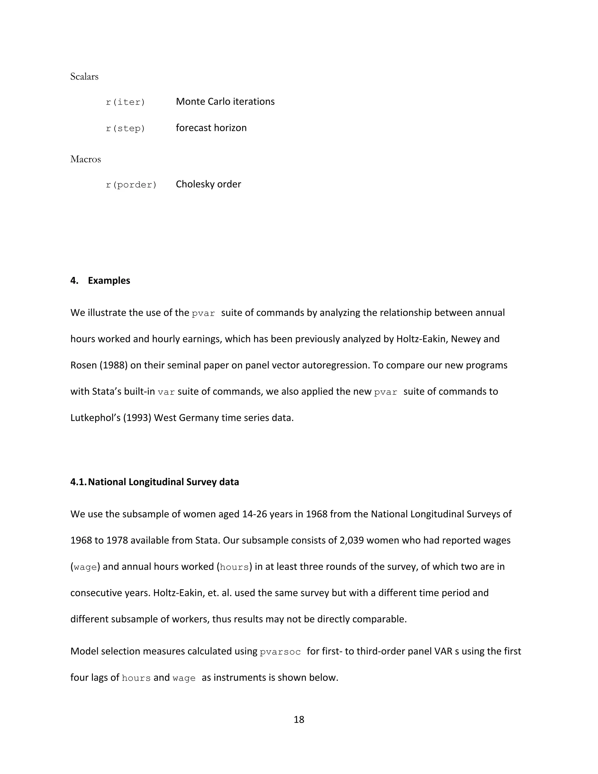
Saved Results
pvarirf saves the following in r():
Scalars
r(iter) Monte Carlo iterations
r(step) forecast horizon
Macros
r(porder) Cholesky order of orthogonalized IRF
3.6.pvarfevd
The post-estimation command pvarfevd computes forecast-error variance decomposition (FEVD)
based on a Cholesky decomposition of the residual covariance matrix of the underlying panel VAR
model. Standard errors and confidence intervals based on Monte Carlo simulation may be optionally
computed.
Caution in interpreting computed FEVD should be exercised when exogenous variables are included in
the underlying panel VAR model. Contributions of exogenous variables, when included in the panel VAR
model, to forecast-error variance are disregarded in calculating FEVD.](https://image.slidesharecdn.com/abrigoandlove2015-171202104944/75/Abrigo-and-love_2015_-17-2048.jpg)
![17
Syntax
pvarfevd [, options]
Options
step(#) specifies the step (forecast) horizon; the default is ten periods.
impulse(impulsevars) and response(responsevars) specify the impulse and response
variables for which forecast-error variance decomposition are to be reported. If impulse() or
response() is not specified, each endogenous variable, in turn, is used.
porder(varlist) specifies the Cholesky ordering of the endogenous variables to be used when
estimating FEVDs. By default, the order in which the variables were originally specified on the
underlying pvar command is used.
mc(#) requests that # Monte Carlo draws be used to estimate the standard errors and the percentile-
based 90% confidence intervals of the FEVDs. Computed standard errors and confidence
intervals are not displayed, but may be saved as a separate file.
dots requests the display of iteration dots. By default, one dot character is displayed for each iteration.
A red 'x' is displayed if the iteration returns an error.
save(filename) specifies that the FEVDs be saved under the name filename. In addition, standard
errors and percentile-based 90% confidence intervals are saved when #>1 in option mc(#) is
specified.
notable requests the table to be constructed but not displayed.
Saved Results
pvarfevd saves the following in r():](https://image.slidesharecdn.com/abrigoandlove2015-171202104944/75/Abrigo-and-love_2015_-18-2048.jpg)
![19
Based on the three model selection criteria by Andrews and Lu (2001) and the over-all coefficient of
determination, first-order panel VAR is the preferred model, since this has the smallest MBIC, MAIC and
MQIC. While we also want to minimize Hansen’s J statistic, it does not correct for the degrees of
freedom in the model like the model and moment selection criteria by Andrews and Lu. Based on the
selection criteria, we fit a first-order panel VAR model with the same specification of instruments as
above using GMM estimation implemented by pvar.
3 .9862297 3.624628 .4591831 -23.29944 -4.375372 -11.62918
2 .988392 5.395145 .7146273 -48.453 -10.60486 -25.11248
1 .9906918 11.74496 .4663737 -69.02726 -12.25504 -34.01648
lag CD J J pvalue MBIC MAIC MQIC
Ave. no. of T = 1.656
No. of panels = 506
Sample: 72 - 73 No. of obs = 838
Selection order criteria
...
Running panel VAR lag order selection on estimation sample
. pvarsoc wage hours, maxlag(3) pvaropts(instl(1/4))
. gen wage = exp(ln_wage)
(National Longitudinal Survey. Young Women 14-26 years of age in 1968)
. webuse nlswork2
Instruments : l(1/4).(wage hours)
L1. .5834965 .1436703 4.06 0.000 .3019079 .865085
hours
L1. -.0575627 .5706831 -0.10 0.920 -1.176081 1.060956
wage
hours
L1. .0170489 .0176144 0.97 0.333 -.0174747 .0515725
hours
L1. .6428702 .0978213 6.57 0.000 .4511439 .8345965
wage
wage
Coef. Std. Err. z P>|z| [95% Conf. Interval]
Ave. no. of T = 1.656
No. of panels = 506
No. of obs = 838
GMM weight matrix: Robust
Initial weight matrix: Identity
Final GMM Criterion Q(b) = .014
GMM Estimation
Panel vector autoregresssion
. pvar wage hours, instl(1/4)](https://image.slidesharecdn.com/abrigoandlove2015-171202104944/75/Abrigo-and-love_2015_-20-2048.jpg)
![20
Note that the 506 women included in the estimation is significantly less than the full subsample of
women available in the data. By default, pvar drops from estimation any observation with missing data.
Since hours worked and wages are not observed in all years for all women in the subsample the number
of observations dropped grows with the lag order of variables included as instruments. We can improve
estimation by using “GMM-style” instruments as proposed by Holtz-Eakin, et. al. Instrument lags with
missing values are replaced with zeroes. This increases the estimation sample, which results to more
efficient estimates.
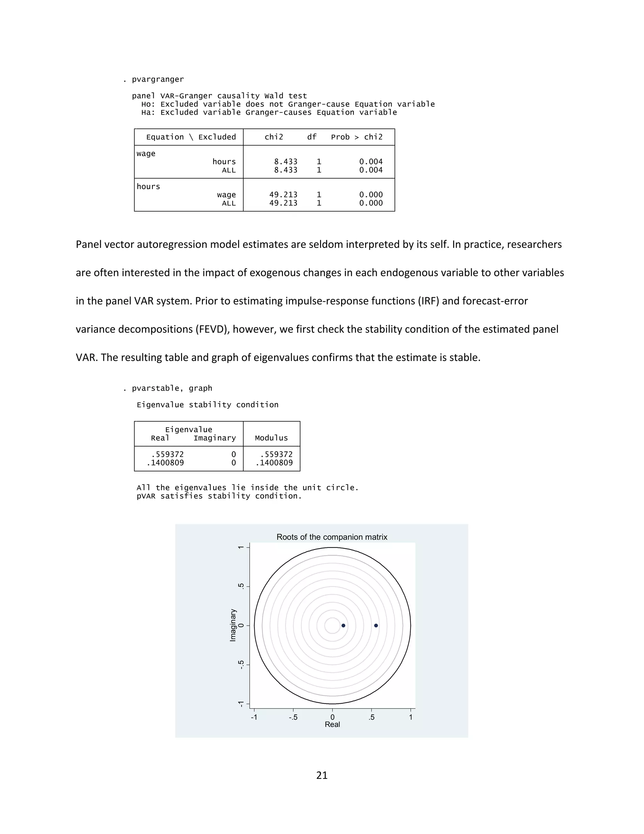
Although Granger causality for a first-order panel VAR may be inferred from the pvar output above, we
still perform the test using pvargranger as an illustration. Results of the Granger causality tests below
show that wage Granger-causes hours, and hours Granger-causes wage at the usual confidence levels,
similar to the findings by Holtz-Eakin, et.al.
Instruments : l(1/4).(wage hours)
L1. -.1068443 .0947648 -1.13 0.260 -.2925799 .0788912
hours
L1. -2.280437 .3250711 -7.02 0.000 -2.917565 -1.643309
wage
hours
L1. .0721378 .0248413 2.90 0.004 .0234498 .1208257
hours
L1. .8062972 .079843 10.10 0.000 .6498078 .9627867
wage
wage
Coef. Std. Err. z P>|z| [95% Conf. Interval]
Ave. no. of T = 2.578
No. of panels = 2039
No. of obs = 5257
GMM weight matrix: Robust
Initial weight matrix: Identity
Final GMM Criterion Q(b) = .00792
GMM Estimation
Panel vector autoregresssion
. pvar wage hours, instl(1/4) gmmstyle](https://image.slidesharecdn.com/abrigoandlove2015-171202104944/75/Abrigo-and-love_2015_-21-2048.jpg)

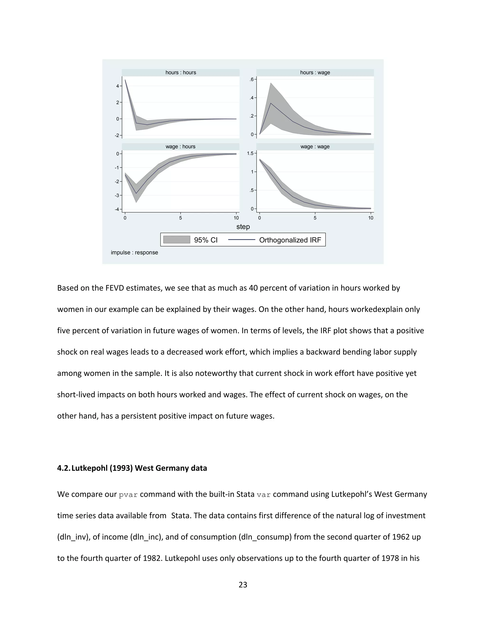


The document describes a Stata package of programs for estimating panel vector autoregression (VAR) models. The package allows for convenient estimation, model selection, inference and other analyses of panel VAR models using generalized method of moments in a Stata environment. The programs address panel VAR specification, estimation, model selection criteria, impulse response analyses, and forecast error variance decomposition. The syntax and outputs of the commands are designed to be similar to Stata's built-in VAR commands for time series data.