Downloaded 1,732 times

![The difference in [whatever the data represents] between sample 1 ( M = 23.241 , VAR = 83.381 ) and sample 2 ( M = 17.597, VAR = 156.742) was statistically significant, t (29) = 1.962, p < .05, one-tailed. 2.045 t Critical two-tail 0.059 P(T<=t) two-tail 1.699 t Critical one-tail 0.030 P(T<=t) one-tail 1.962 t Stat 29.000 df 0.000 Hypothesised Mean Difference -0.036 Pearson Correlation 30.000 30.000 Observations 156.742 83.381 Variance 17.597 23.241 Mean sample 2 sample 1 t-Test: Paired Two Sample for Means](https://image.slidesharecdn.com/t-test-101229084129-phpapp02/75/Introduction-to-t-tests-statistics-18-2048.jpg)

The document discusses different types of t-tests used to determine if the means of two samples are statistically significantly different from each other. It describes paired sample t-tests used to compare means when the same subjects are measured before and after a treatment. It also describes two-sample t-tests used to compare independent samples that may have equal or unequal variances, and whether the tests are one-tailed or two-tailed. Examples are provided of interpreting t-test output and determining if differences are statistically significant based on the t-statistic and p-values. Non-parametric alternatives like the Mann-Whitney U test are also briefly mentioned.
Overview of t-tests presented by Dr. Bryan Mills.
Defining the reasons for using t-tests in statistical analysis.
Application of t-tests when comparing two sets of data with normal distributions.
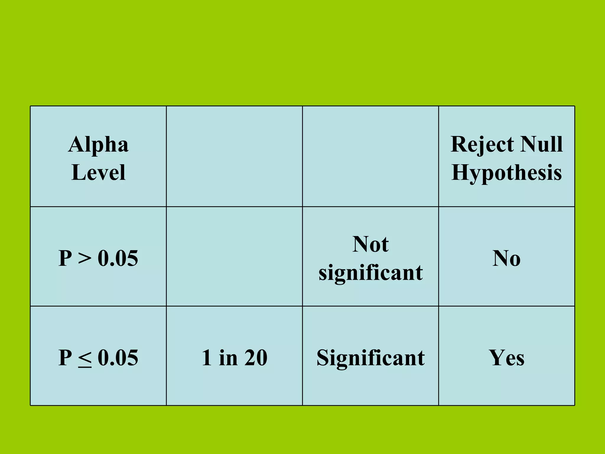
A low p-value indicates a significant result, traditionally p < 0.05.
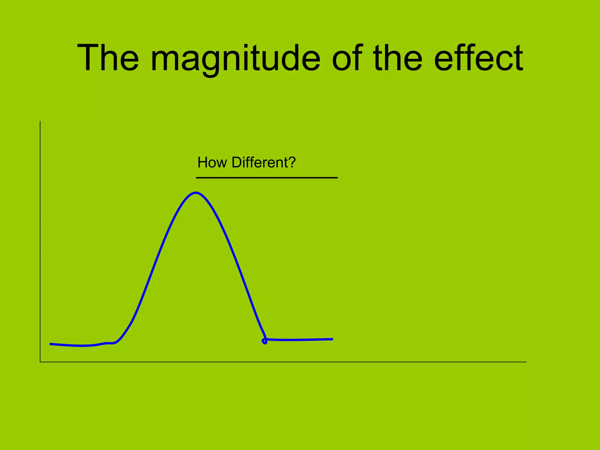
Discussion on how to assess the magnitude of differences between datasets.
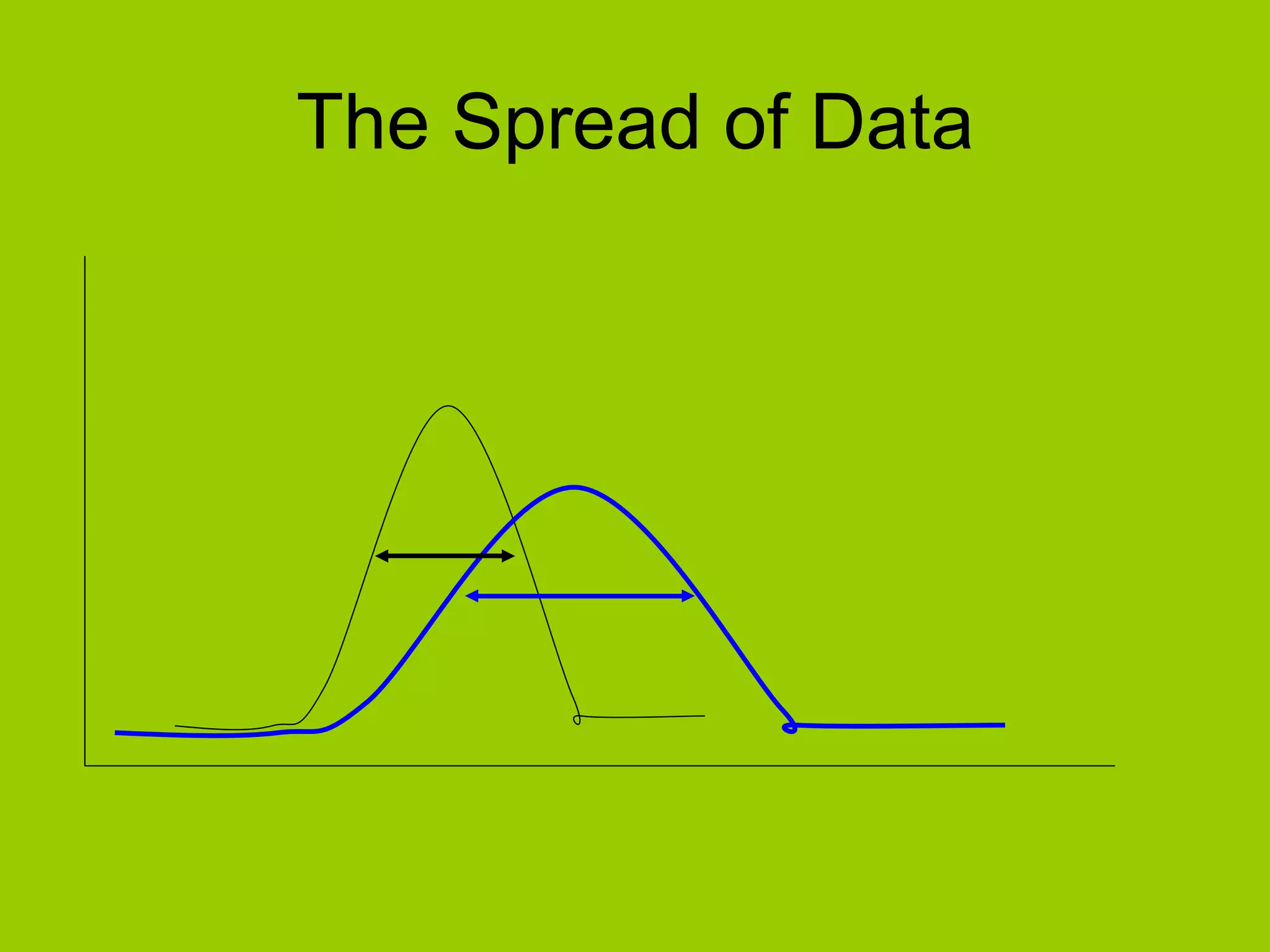
Emphasizes the importance of understanding the spread of the data being analyzed.
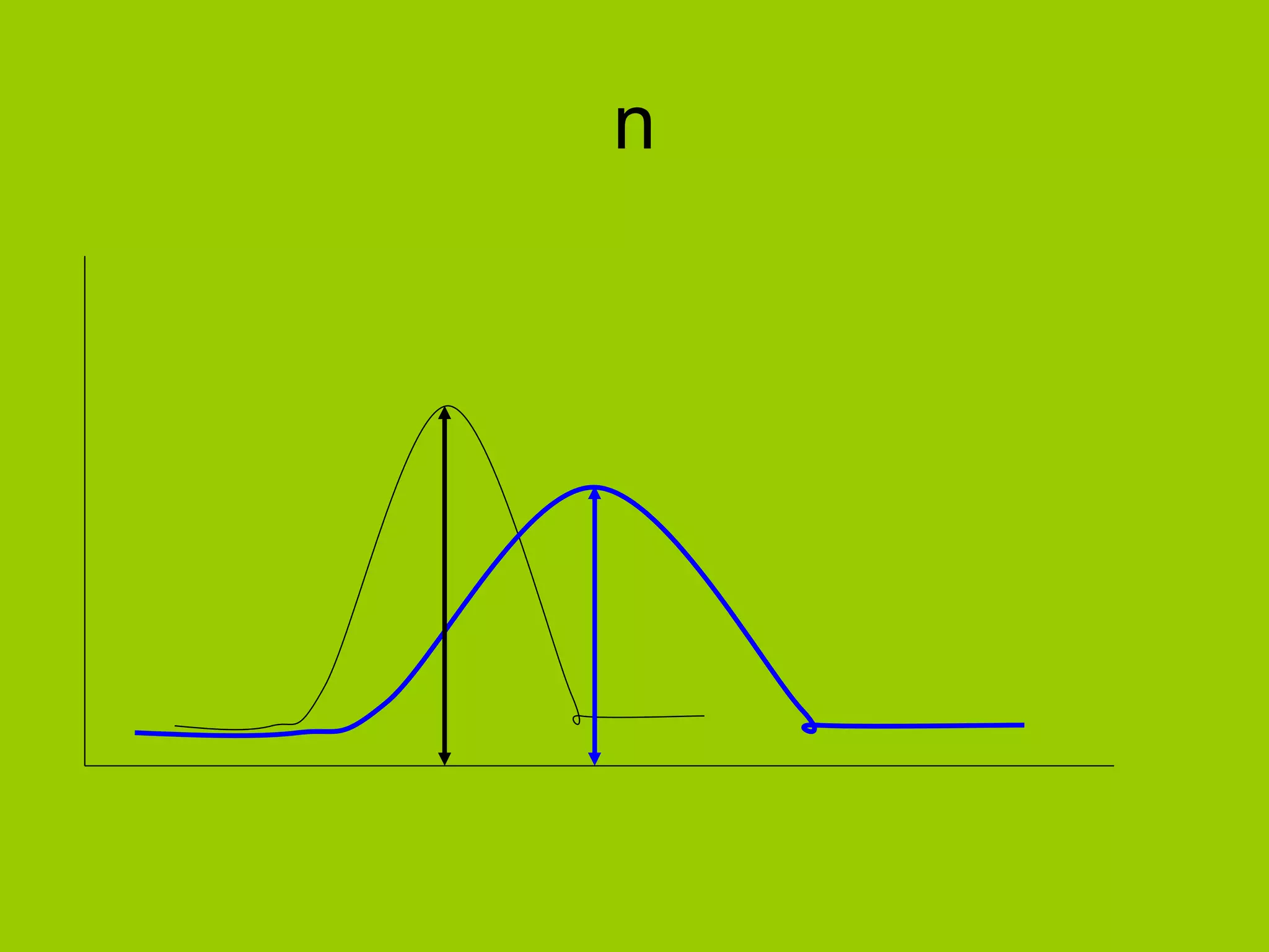
Introduces statistical notation 'n' referring to sample size.
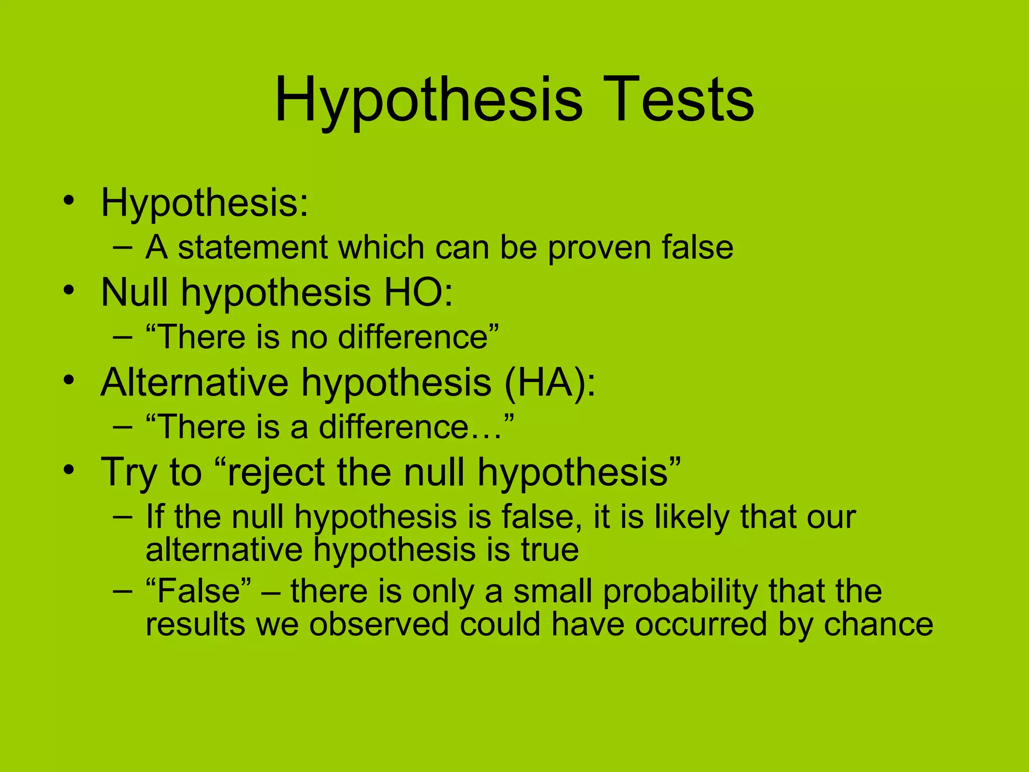
Defines null and alternative hypotheses, aimed at rejecting the null hypothesis for significance.
Criteria for accepting or rejecting the null hypothesis based on p-value thresholds.
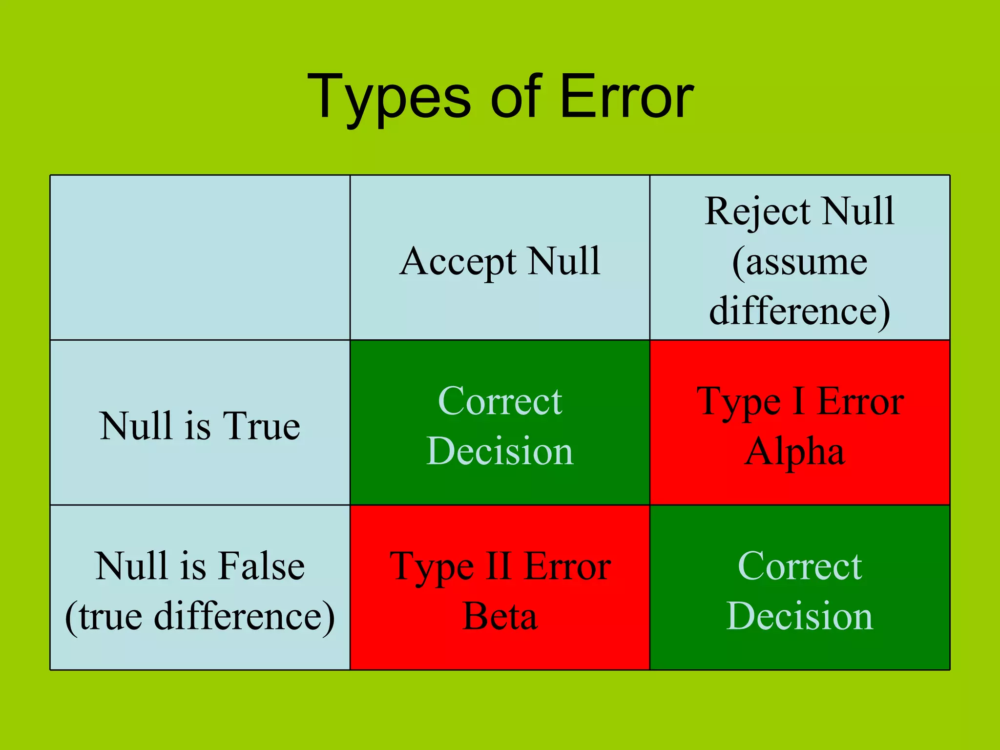
Explains Type I and Type II errors in hypothesis testing and their implications.
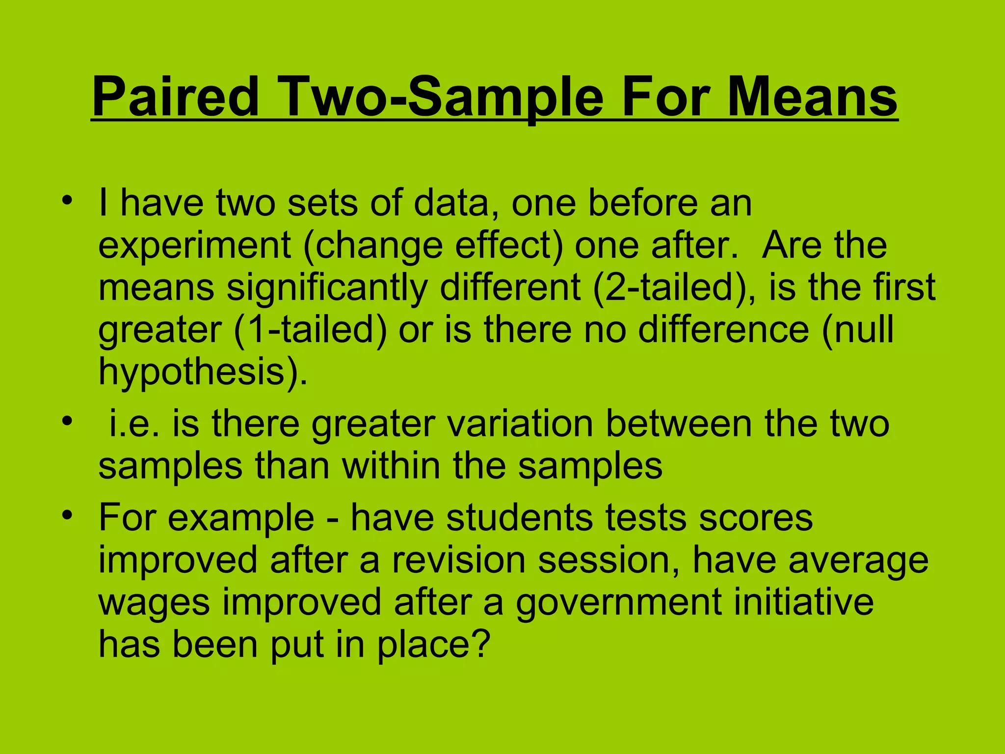
Looks at paired t-tests for before-and-after comparisons in experiments.
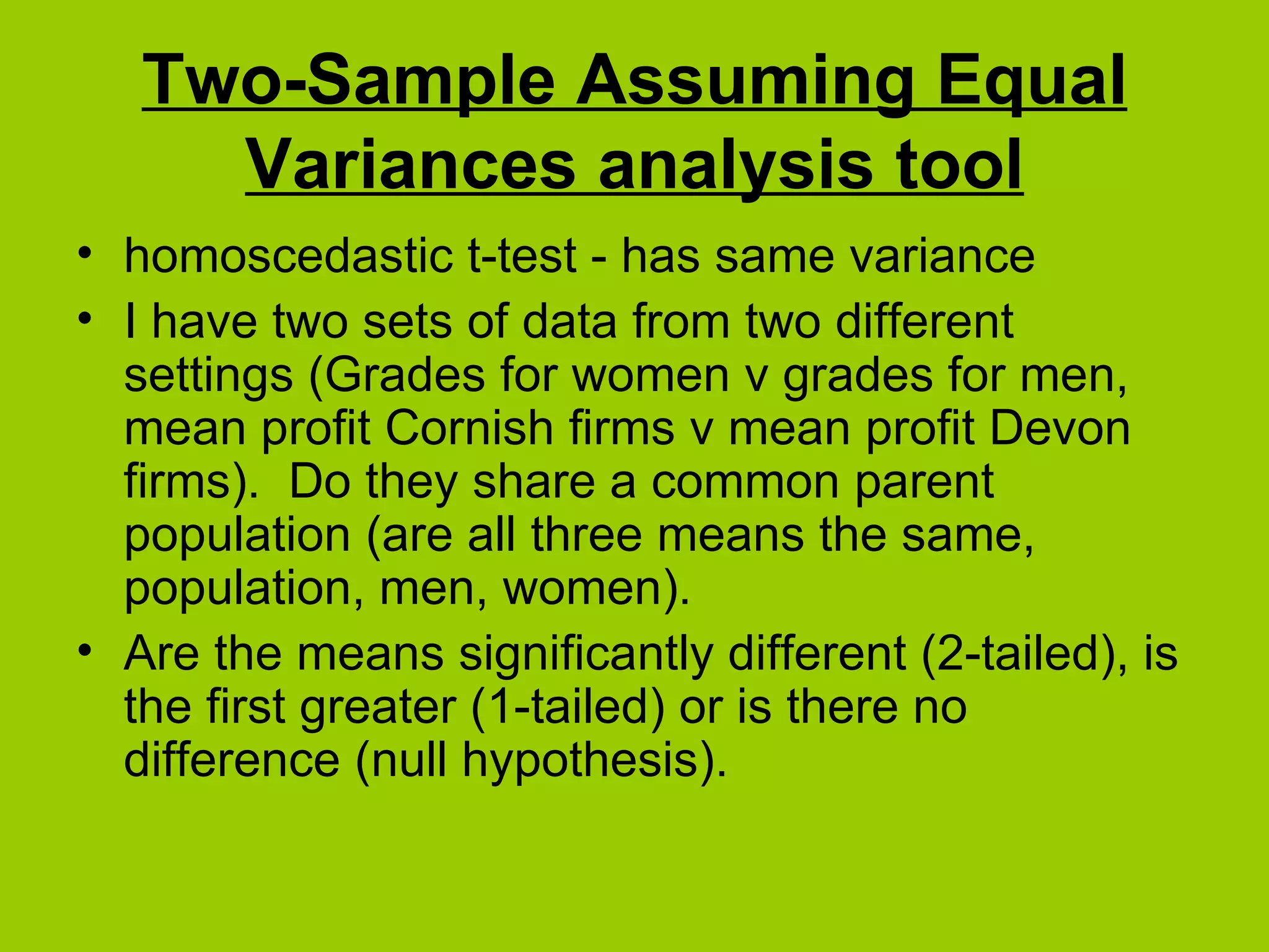
Two-sample t-test assuming equal variances for various datasets.
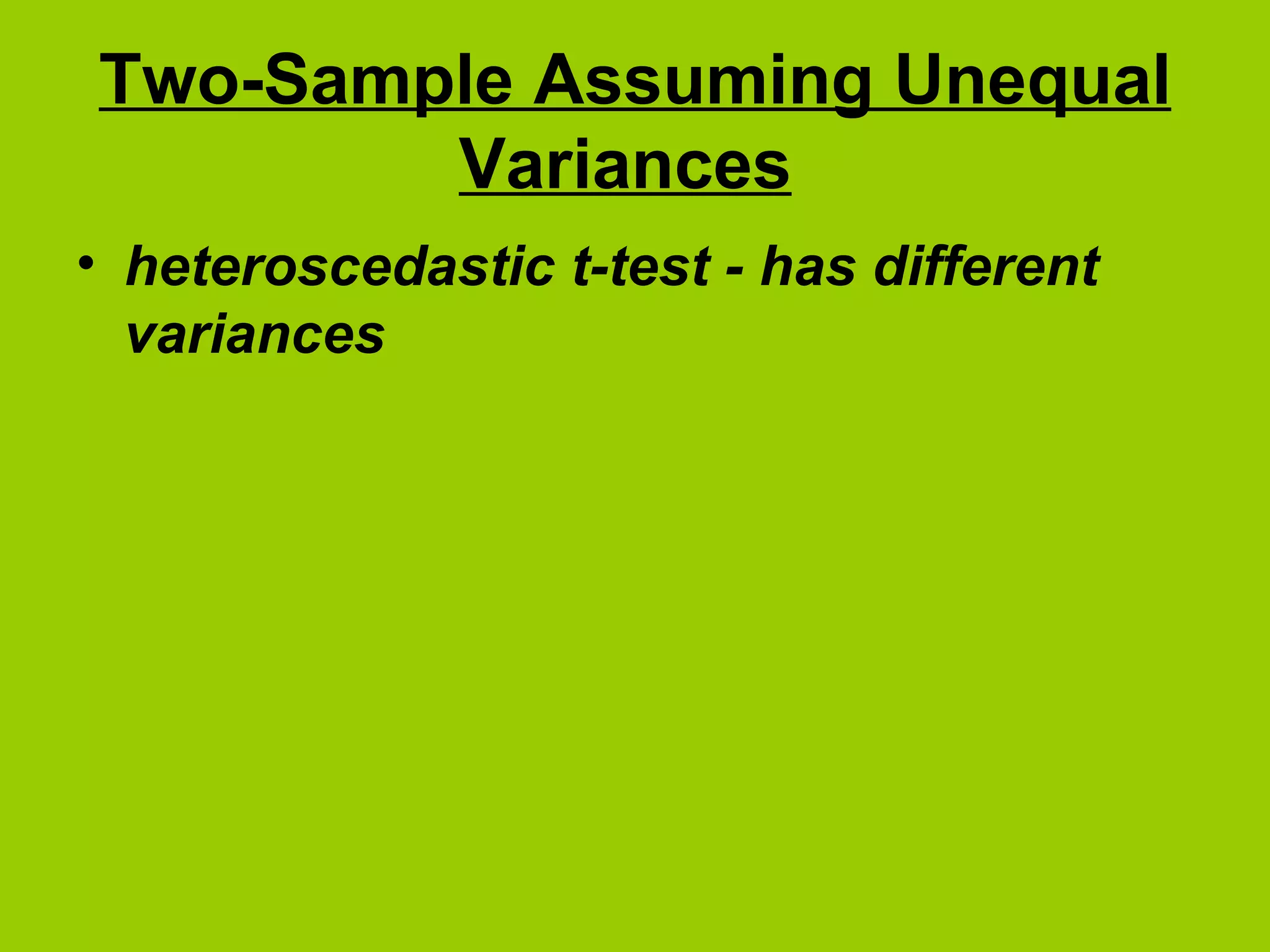
Two-sample t-test handling situations with unequal variances.
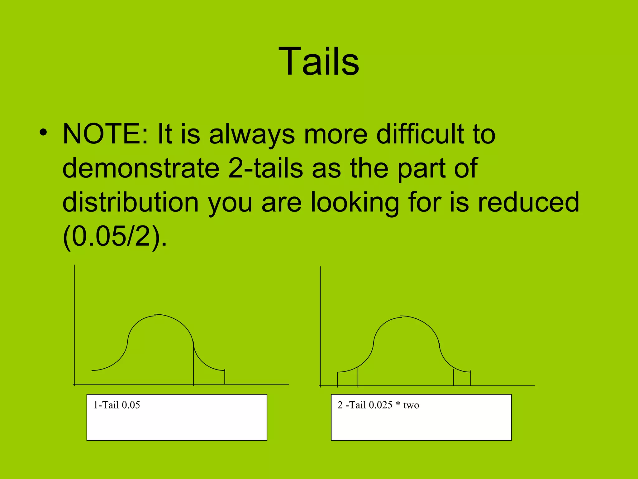
Explains the concept of one-tailed vs two-tailed tests and their probability allocations.
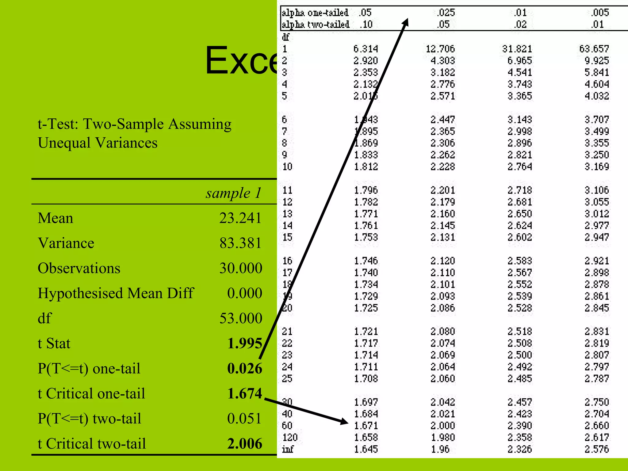
How to interpret the t-test output from Excel for further analysis.
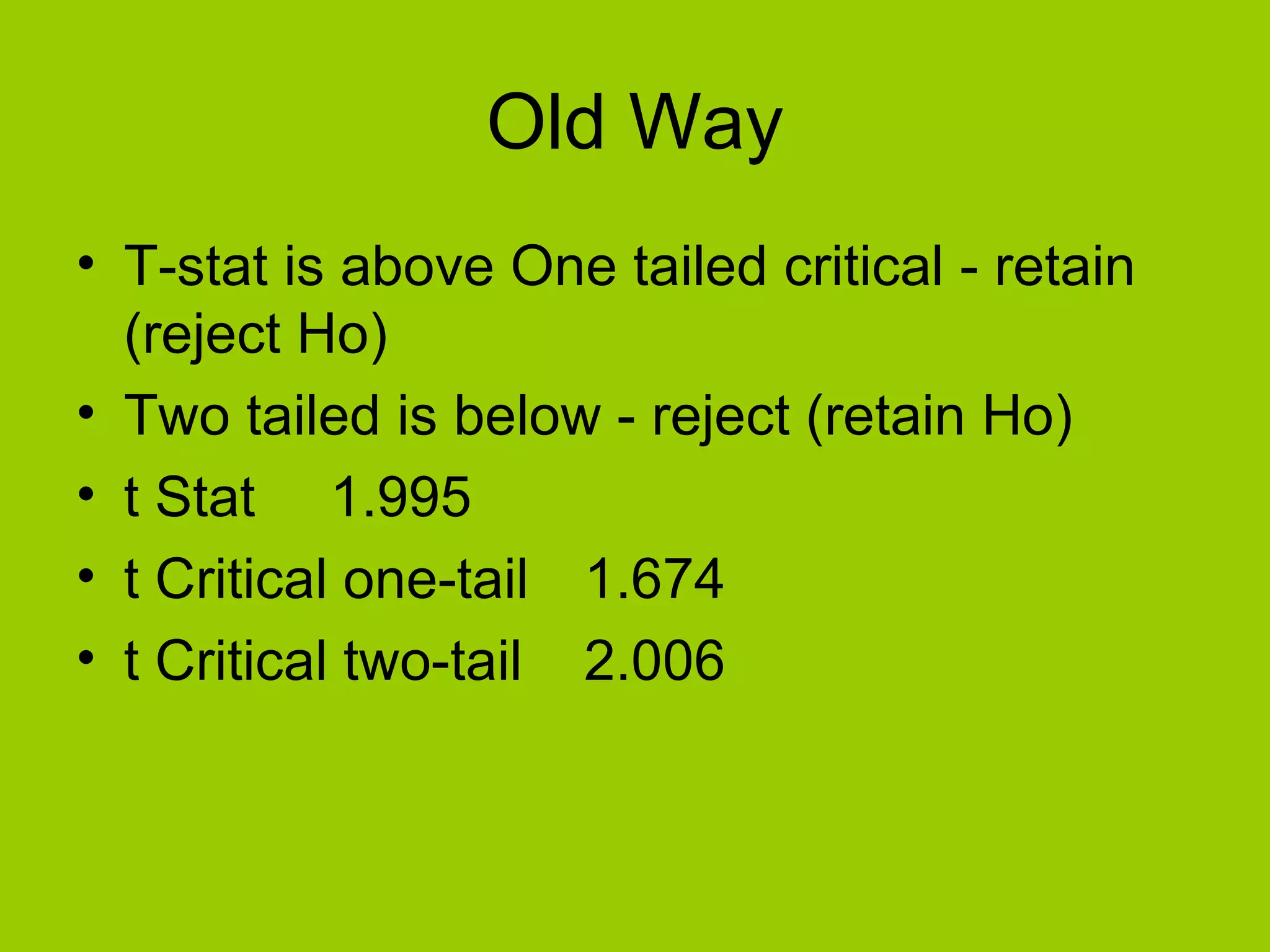
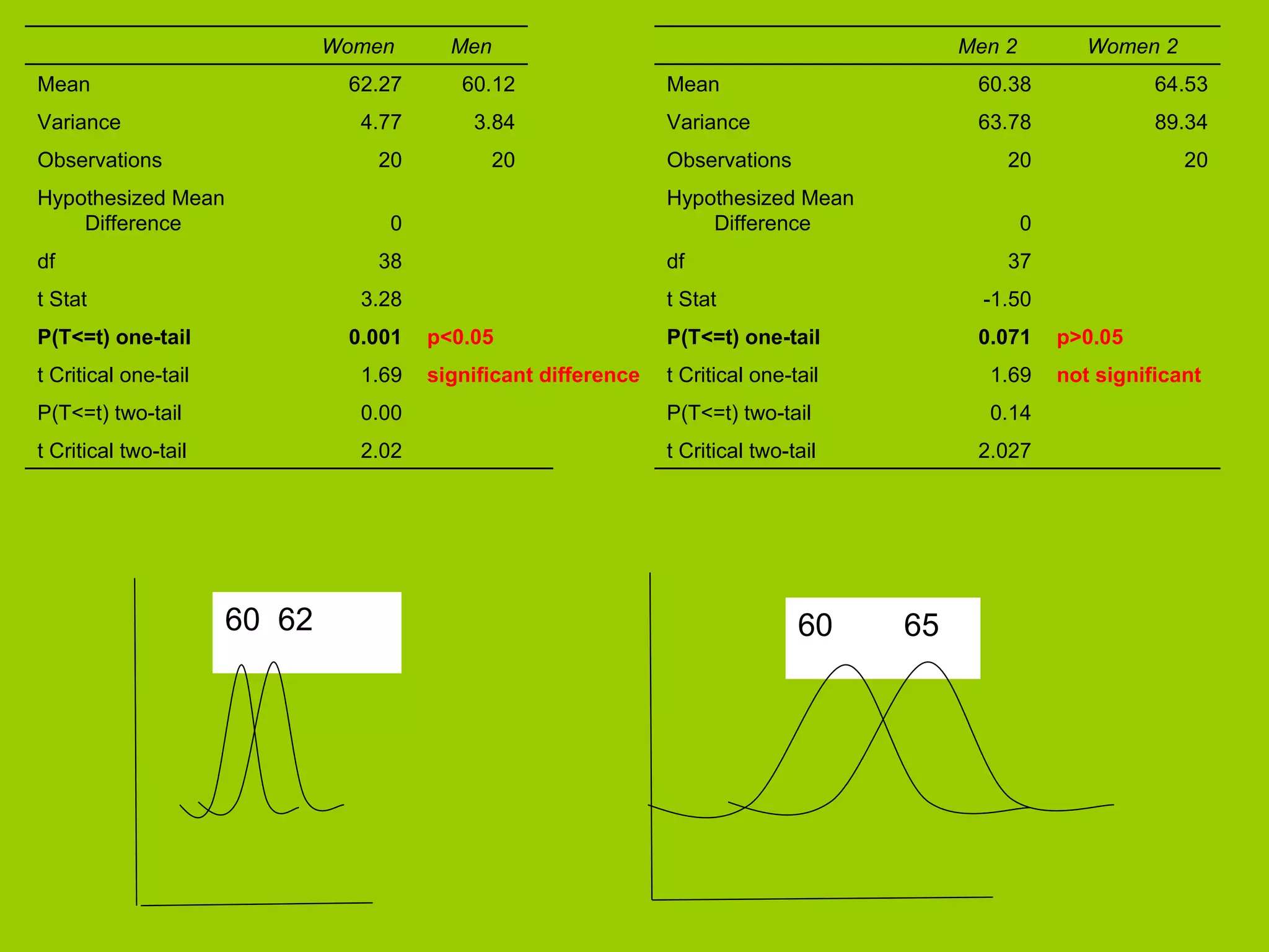
Comparing t-statistics against critical values to decide on hypotheses.
Detailed analysis of statistical significance using sample data and variance.
Demonstrates a significant difference in sample comparisons with statistical evidence.
Introduction to non-parametric tests like Mann-Whitney U test as alternatives.
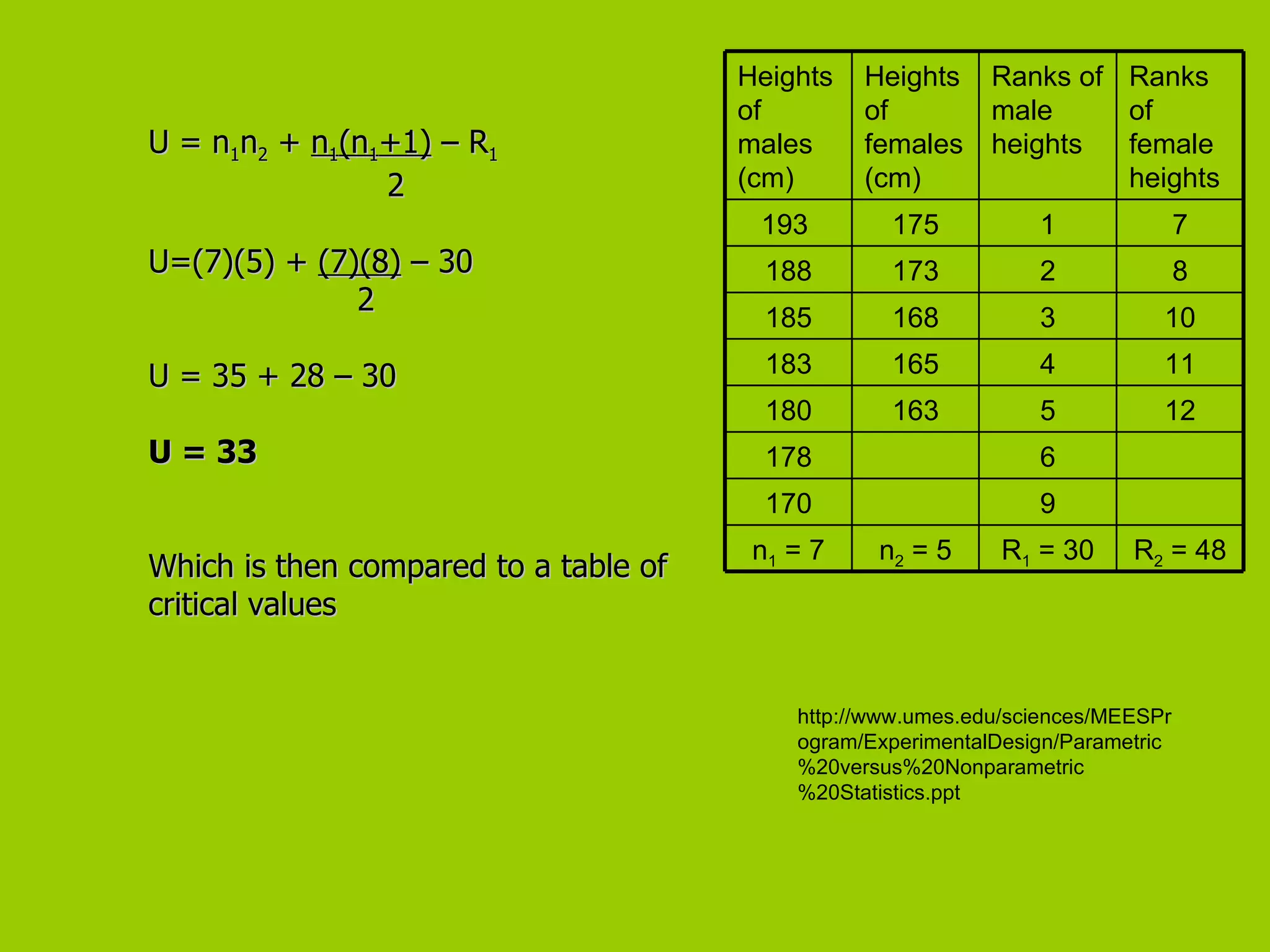
Detailed calculation for Mann-Whitney U test and its comparison to critical values.