BASIC STATISTICS

1. Workshop on Data Analysis for Management
and Social Sciences
Dr. Madhanrajan Udayanan

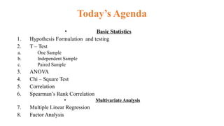
2. Today’s Agenda
• Basic Statistics
1. Hypothesis Formulation and testing
2. T – Test
a. One Sample
b. Independent Sample
c. Paired Sample
3. ANOVA
4. Chi – Square Test
5. Correlation
6. Spearman’s Rank Correlation
• Multivariate Analysis
7. Multiple Linear Regression
8. Factor Analysis

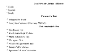
3. Measures of Central Tendency
 Mean
 Median
 Mode
Parametric Test
 Independent T-test
 Analysis of variance (One-way ANOVA)
Non Parametric Test
 Friedman's Test
 Kruskal-Wallis (KW) Test
 Mann-Whitney U Test
 Chi square Test
 Wilcoxon Signed rank Test
 Pearson’s Correlation
 Spearman’s Rank Correlation

5. DEVELOPING HYPOTHESIS
AND
RESEARCH QUESTIONS

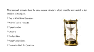
6. Most research projects share the same general structure, which could be represented in the
shape of an hourglass .
Beg In With Broad Questions
Narrow Down, Focus In
Operationalize
Observe
Analyze Data
Reach Conclusions
Generalize Back To Questions

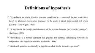
7. Definitions of hypothesis
 “Hypotheses are single tentative guesses, good hunches – assumed for use in devising
theory or planning experiments intended to be given a direct experimental test when
possible”. (Eric Rogers, 1966 )
 “A hypothesis is a conjectural statement of the relation between two or more variables”.
(Kerlinger, 1956)
 “Hypothesis is a formal statement that presents the expected relationship between an
independent and dependent variable.”(Creswell, 1994)
 “A research question is essentially a hypothesis asked in the form of a question.”

8. Nature of Hypothesis
 It can be tested – verifiable or falsifiable.
 Hypotheses are not moral or ethical questions.
 It is neither too specific nor to general.
 It is a prediction of consequences.
 It is considered valuable even if proven false.

9. Types of Hypotheses
The null hypothesis represents a theory that has been put forward, either because it
is believed to be true or because it is to be used as a basis for argument, but has not
been proved.
Has serious outcome if incorrect decision is made!
The alternative hypothesis is a statement of what a hypothesis test is set up to
establish.
 Opposite of Null Hypothesis.
 Only reached if H0 is rejected.
 Frequently “alternative” is actual desired conclusion of the researcher!

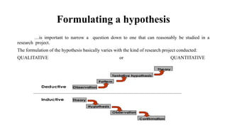
10. Formulating a hypothesis
…is important to narrow a question down to one that can reasonably be studied in a
research project.
The formulation of the hypothesis basically varies with the kind of research project conducted:
QUALITATIVE or QUANTITATIVE

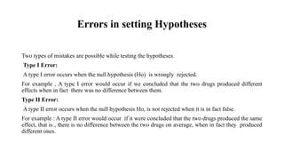
11. Errors in setting Hypotheses
Two types of mistakes are possible while testing the hypotheses.
Type I Error:
A type I error occurs when the null hypothesis (Ho) is wrongly rejected.
For example , A type I error would occur if we concluded that the two drugs produced different
effects when in fact there was no difference between them.
Type II Error:
A type II error occurs when the null hypothesis Ho, is not rejected when it is in fact false.
For example : A type II error would occur if it were concluded that the two drugs produced the same
effect, that is , there is no difference between the two drugs on average, when in fact they produced
different ones.

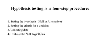
12. Hypothesis testing is a four-step procedure:
1. Stating the hypothesis (Null or Alternative)
2. Setting the criteria for a decision
3. Collecting data
4. Evaluate the Null hypothesis

13. Example of How Theory plays a role
in
Hypothesis framing

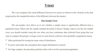
15. T-test
The t-test compares the actual difference between two means in relation to the variation in the data
(expressed as the standard deviation of the difference between the means).
One-Sample T-test
The one-sample t-test allows us to test whether a sample mean is significantly different from a
population mean. When only the sample standard deviation is known. Simply, when to use the one-sample
t-test, you should consider using this test when you have continuous data collected from group that you
want to compare that group’s average scores to some known criterion value (probably a population mean).
 Often performed for testing the mean value of distribution.
 It can be used under the assumption that sample distribution is normal.
 For large samples, the procedure performs often well even for non-normal population.

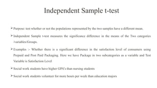
16. Independent Sample t-test
Purpose: test whether or not the populations represented by the two samples have a different mean.
Independent Sample t-test measures the significance difference in the means of the Two categories
/variables/Groups.
Examples :- Whether there is a significant difference in the satisfaction level of consumers using
Prepaid and Post Paid Packaging. Here we have Package in two subcategories as a variable and Test
Variable is Satisfaction Level
Social work students have higher GPA’s than nursing students
Social work students volunteer for more hours per week than education majors

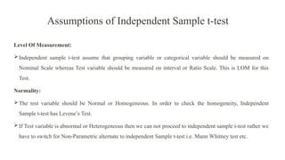
17. Assumptions of Independent Sample t-test
Level Of Measurement:
Independent sample t-test assume that grouping variable or categorical variable should be measured on
Nominal Scale whereas Test variable should be measured on interval or Ratio Scale. This is LOM for this
Test.
Normality:
The test variable should be Normal or Homogeneous. In order to check the homogeneity, Independent
Sample t-test has Levene’s Test.
If Test variable is abnormal or Heterogeneous then we can not proceed to independent sample t-test rather we
have to switch for Non-Parametric alternate to independent Sample t-test i.e. Mann Whitney test etc.

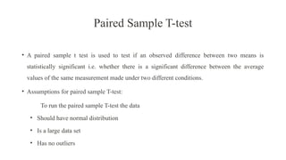
18. Paired Sample T-test
• A paired sample t test is used to test if an observed difference between two means is
statistically significant i.e. whether there is a significant difference between the average
values of the same measurement made under two different conditions.
• Assumptions for paired sample T-test:
To run the paired sample T-test the data
• Should have normal distribution
• Is a large data set
• Has no outliers

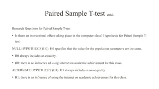
19. Research Questions for Paired Sample T-test
• Is there an instructional effect taking place in the computer class? Hypothesis for Paired Sample T-
test:
NULL HYPOTHESIS (H0): H0 specifies that the value for the population parameters are the same.
• H0 always includes an equality.
• H0: there is no influence of using internet on academic achievement for this class.
ALTERNATE HYPOTHESIS (H1): H1 always includes a non-equality
• H1: there is an influence of using the internet on academic achievement for this class.
Paired Sample T-test cntd..

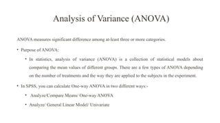
20. Analysis of Variance (ANOVA)
ANOVA measures significant difference among at-least three or more categories.
• Purpose of ANOVA:
• In statistics, analysis of variance (ANOVA) is a collection of statistical models about
comparing the mean values of different groups. There are a few types of ANOVA depending
on the number of treatments and the way they are applied to the subjects in the experiment.
• In SPSS, you can calculate One-way ANOVA in two different ways:-
• Analyze/Compare Means/ One-way ANOVA
• Analyze/ General Linear Model/ Univariate

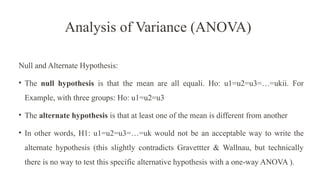
21. Analysis of Variance (ANOVA)
Null and Alternate Hypothesis:
• The null hypothesis is that the mean are all equali. Ho: u1=u2=u3=…=ukii. For
Example, with three groups: Ho: u1=u2=u3
• The alternate hypothesis is that at least one of the mean is different from another
• In other words, H1: u1=u2=u3=…=uk would not be an acceptable way to write the
alternate hypothesis (this slightly contradicts Gravettter & Wallnau, but technically
there is no way to test this specific alternative hypothesis with a one-way ANOVA ).

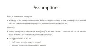
22. Assumptions
Level of Measurement assumption:
• According to this assumption one variable should be categorical having at least 3-subcategories or nominal
scale and Test variable (dependent) should be measured on interval or Ratio Scale.
Normality:
• Second assumption is Normality or Homogeneity of the Test variable. This means that the test variable
should be normal and we test this by means of Levene’s Test.
• The Hypothesis of ANOVA are
• Null : means across the categories are equal
• Alternate: means across the categories are not equal

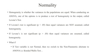
23. Normality
• Homogeneity is whether the variances in the populations are equal. When conducting an
ANOVA, one of the options is to produce a test of homogeneity in the output, called
Levene’s Test.
• If Levene’s test is significant (p < .05) then equal variances are NOT assumed, called
heterogeneity.
• If Levene’s is not significant (p > .05) then equal variances are assumed, called
homogeneity.
• What if
• If Test variable is not Normal, then we switch to the Non-Parametric alternate to
ANOVA i.e. Kruskal Wallis Test…

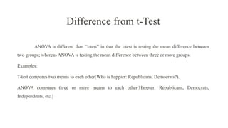
24. Difference from t-Test
ANOVA is different than “t-test” in that the t-test is testing the mean difference between
two groups; whereas ANOVA is testing the mean difference between three or more groups.
Examples:
T-test compares two means to each other(Who is happier: Republicans, Democrats?).
ANOVA compares three or more means to each other(Happier: Republicans, Democrats,
Independents, etc.)

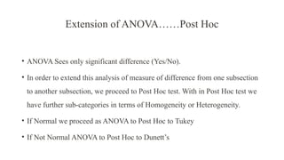
25. Extension of ANOVA……Post Hoc
• ANOVA Sees only significant difference (Yes/No).
• In order to extend this analysis of measure of difference from one subsection
to another subsection, we proceed to Post Hoc test. With in Post Hoc test we
have further sub-categories in terms of Homogeneity or Heterogeneity.
• If Normal we proceed as ANOVA to Post Hoc to Tukey
• If Not Normal ANOVA to Post Hoc to Dunett’s

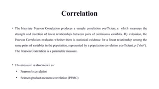
26. Correlation
• The bivariate Pearson Correlation produces a sample correlation coefficient, r, which measures the
strength and direction of linear relationships between pairs of continuous variables. By extension, the
Pearson Correlation evaluates whether there is statistical evidence for a linear relationship among the
same pairs of variables in the population, represented by a population correlation coefficient, ρ (“rho”).
The Pearson Correlation is a parametric measure.
• This measure is also known as:
• Pearson’s correlation
• Pearson product-moment correlation (PPMC)

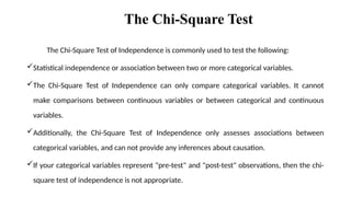
27. The Chi-Square Test
The Chi-Square Test of Independence is commonly used to test the following:
Statistical independence or association between two or more categorical variables.
The Chi-Square Test of Independence can only compare categorical variables. It cannot
make comparisons between continuous variables or between categorical and continuous
variables.
Additionally, the Chi-Square Test of Independence only assesses associations between
categorical variables, and can not provide any inferences about causation.
If your categorical variables represent "pre-test" and "post-test" observations, then the chi-
square test of independence is not appropriate.

28. Welcome Back

29. Regression: Introduction
Basic idea:
Use data to identify relationships among
variables and use these relationships to make
predictions.

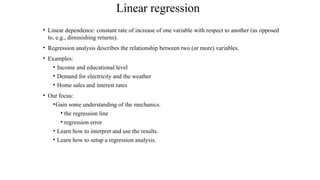
30. Linear regression
• Linear dependence: constant rate of increase of one variable with respect to another (as opposed
to, e.g., diminishing returns).
• Regression analysis describes the relationship between two (or more) variables.
• Examples:
• Income and educational level
• Demand for electricity and the weather
• Home sales and interest rates
• Our focus:
•Gain some understanding of the mechanics.
• the regression line
• regression error
• Learn how to interpret and use the results.
• Learn how to setup a regression analysis.

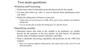
31. Two main questions:
•Prediction and Forecasting
• Predict home sales for December given the interest rate for this month.
• Use time series data (e.g., sales vs. year) to forecast future performance (next
year sales).
• Predict the selling price of houses in some area.
• Collect data on several houses (# of BR, #BA, sq.ft, lot size, property tax) and their
selling price.
• Can we use this data to predict the selling price of a specific house?
•Quantifying causality
• Determine factors that relate to the variable to be predicted; e.g., predict
growth for the economy in the next quarter: use past history on quarterly
growth, index of leading economic indicators, and others.
• Want to determine advertising expenditure and promotion for the 1999 Ford
Explorer.
•Sales over a quarter might be influenced by: ads in print, ads in radio, ads in TV, and
other promotions.

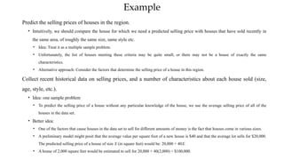
32. Example
Predict the selling prices of houses in the region.
• Intuitively, we should compare the house for which we need a predicted selling price with houses that have sold recently in
the same area, of roughly the same size, same style etc.
• Idea: Treat it as a multiple sample problem.
• Unfortunately, the list of houses meeting these criteria may be quite small, or there may not be a house of exactly the same
characteristics.
• Alternative approach: Consider the factors that determine the selling price of a house in this region.
Collect recent historical data on selling prices, and a number of characteristics about each house sold (size,
age, style, etc.).
• Idea: one sample problem
• To predict the selling price of a house without any particular knowledge of the house, we use the average selling price of all of the
houses in the data set.
• Better idea:
• One of the factors that cause houses in the data set to sell for different amounts of money is the fact that houses come in various sizes.
• A preliminary model might posit that the average value per square foot of a new house is $40 and that the average lot sells for $20,000.
The predicted selling price of a house of size X (in square feet) would be: 20,000 + 40X.
• A house of 2,000 square feet would be estimated to sell for 20,000 + 40(2,000) = $100,000.

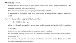
33. •Probability Model:
• We know, however, that this is just an approximation, and the selling price of this particular house of 2,000
square feet is not likely to be exactly $100,000.
• Prices for houses of this size may actually range from $50,000 to $150,000.
• In other words, the deterministic model is not really suitable. We should therefore consider a probabilistic
model.
•Let Y be the actual selling price of the house. Then
Y = 20,000 + 40x + ,
where  (Greek letter epsilon) represents a random error term (which might be positive
or negative).
• If the error term  is usually small, then we can say the model is a good one.
• The random term, in theory, accounts for all the variables that are not part of the model (for instance, lot size,
neighborhood, etc.).
• The value of  will vary from sale to sale, even if the house size remains constant. That is, houses of the
exact same size may sell for different prices.

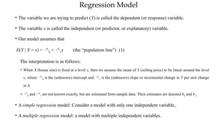
34. Regression Model
• The variable we are trying to predict (Y) is called the dependent (or response) variable.
• The variable x is called the independent (or predictor, or explanatory) variable.
• Our model assumes that
E(Y | X = x) = 0
+ 1
x (the “population line”) (1)
The interpretation is as follows:
• When X (house size) is fixed at a level x, then we assume the mean of Y (selling price) to be linear around the level
x, where 0
is the (unknown) intercept and 1
is the (unknown) slope or incremental change in Y per unit change
in X.
• 0
and 1
are not known exactly, but are estimated from sample data. Their estimates are denoted b0
and b1
.
• A simple regression model: Consider a model with only one independent variable,.
• A multiple regression model: a model with multiple independent variables.

35. House Number Y: Actual Selling
Price ($1,000s)
X: House Size (100s ft2)
1 89.5 20.0
2 79.9 14.8
3 83.1 20.5
4 56.9 12.5
5 66.6 18.0
6 82.5 14.3
7 126.3 27.5
8 79.3 16.5
9 119.9 24.3
10 87.6 20.2
11 112.6 22.0
12 120.8 .019
13 78.5 12.3
14 74.3 14.0
15 74.8 16.7
Averages 88.84 18.17
Sample 15
houses from
the region.

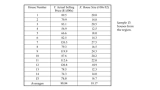
36. Making Inferences about Coefficients
• To assess the accuracy of the model, it involves determining whether a particular
variable like house size has any effect on the selling price.
•Suppose that when a regression line is drawn it produces a horizontal line. This means the selling
price of the house is unaffected by the size of the house.
•A horizontal line has a slope of 0, so when no linear relationship exists between an independent
variable and the dependent variable we should expect to get 1
= 0.
•But of course, we only observe estimate of 1
, which might only be “close” to zero. To
systematically determine when 1
might in fact be zero, we will make inferences about it using
our estimate , specifically, we will do hypothesis tests and build confidence intervals.
• Testing 1
, we can test any of the following:
•H0
: 1
= 0 versus HA
: 1
 0
•H0
: 1
 0 versus HA
: 1
< 0
•H0
: 1
 0 versus HA
: 1
> 0
• In each case, the null hypothesis can be reduced to H0
: 1
= 0. The test statistic in
each case is   1
ˆ
1 /
0
ˆ

 s


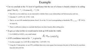
37. Example
• Can we conclude at the 1% level of significance that the size of a house is linearly related to its selling
price? Test H0
: 1
= 0 versus HA
: 1
 0
• Note this is a two-sided test, we are interested in whether there is any relationship at all between price and size.
• Calculate T = (3.879 - 0) / 0.794 = 4.88.
• That is, we are 4.88 standard deviations from 0. So at the 1% level (corresponding to thresholds  t(13, 0.005)
=  3.012),
we reject H0
.
• There is sufficient evidence to conclude that house size does linearly affect selling price.
• To get a p-value on this we would need to look up 4.88 inside the t-table.
• It is 0.00024 or 0.024%; very small indeed.
• A 95% confidence interval for 1
is given by
• For this example: It is 3.879  (2.160)(0.794) = 3.879  1.715.
• Using the 15 data points, we are 95% confident that every extra square foot increases the price of the house by anywhere
from $21.64 to $55.94.
1
ˆ
)
025
.
0
,
2
(
1
ˆ

 s
t n


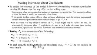
38. Regression Statistics
• Define R2
= SSR/SST = 1- SSE/SST
• The fraction of the total variation explained by the regression.
• R2
is a measure of the explanatory power of the model.
• Multiple-R = (R2
)1/2
(in one variable case = |rXY|)
• According to the definition of R2
, adding extraneous explanatory variables will artificially inflate the R2
.
• We must be careful in interpreting this number.
• Introducing extra variables can lead to spurious results and can interfere with the proper estimation of slopes for the
important variables.
• In order to penalize an excess of variables, we consider the adjusted R2
, which is
adjusted R2
= 1- [SSE/(n-k-1)]/[SST/(n-1)] .
Here n is the number of data and k is the number of explanatory variables.
• The adjusted R2
thus divides numerator and denominator by their DF.

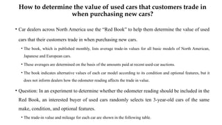
39. How to determine the value of used cars that customers trade in
when purchasing new cars?
• Car dealers across North America use the “Red Book” to help them determine the value of used
cars that their customers trade in when purchasing new cars.
• The book, which is published monthly, lists average trade-in values for all basic models of North American,
Japanese and European cars.
• These averages are determined on the basis of the amounts paid at recent used-car auctions.
• The book indicates alternative values of each car model according to its condition and optional features, but it
does not inform dealers how the odometer reading affects the trade in value.
• Question: In an experiment to determine whether the odometer reading should be included in the
Red Book, an interested buyer of used cars randomly selects ten 3-year-old cars of the same
make, condition, and optional features.
• The trade-in value and mileage for each car are shown in the following table.

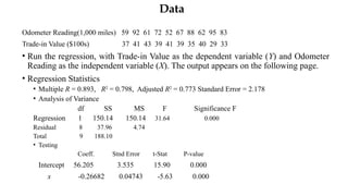
40. Data
Odometer Reading(1,000 miles) 59 92 61 72 52 67 88 62 95 83
Trade-in Value ($100s) 37 41 43 39 41 39 35 40 29 33
• Run the regression, with Trade-in Value as the dependent variable (Y) and Odometer
Reading as the independent variable (X). The output appears on the following page.
• Regression Statistics
• Multiple R = 0.893, R2
= 0.798, Adjusted R2
= 0.773 Standard Error = 2.178
• Analysis of Variance
df SS MS F Significance F
Regression 1 150.14 150.14 31.64 0.000
Residual 8 37.96 4.74
Total 9 188.10
• Testing
Coeff. Stnd Error t-Stat P-value
Intercept 56.205 3.535 15.90 0.000
x -0.26682 0.04743 -5.63 0.000

41. F and F-significance
• F is a test statistic testing whether the estimated model is meaningful; i.e.,
statistically significant.
•F =MSR/MSE
•A large F or a small p-value (or F-significance) implies that the model is significant.
•It is unusual not to reject this null hypothesis.

42. Factor Analysis
• Factor analysis is a class of procedures used for data reduction and summarization.
• It is an interdependence technique: no distinction between dependent and
independent variables.
• Factor analysis is used:
• To identify underlying dimensions, or factors, that explain the correlations
among a set of variables.
• To identify a new, smaller, set of uncorrelated variables to replace the original set
of correlated variables.

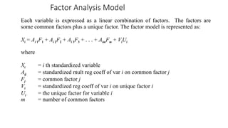
43. Factor Analysis Model
Each variable is expressed as a linear combination of factors. The factors are
some common factors plus a unique factor. The factor model is represented as:
Xi = Ai 1F1 + Ai 2F2 + Ai 3F3 + . . . + AimFm + ViUi
where
Xi = i th standardized variable
Aij = standardized mult reg coeff of var i on common factor j
Fj = common factor j
Vi = standardized reg coeff of var i on unique factor i
Ui = the unique factor for variable i
m = number of common factors

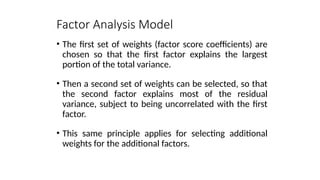
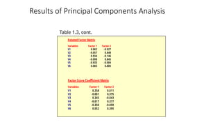
44. • The first set of weights (factor score coefficients) are
chosen so that the first factor explains the largest
portion of the total variance.
• Then a second set of weights can be selected, so that
the second factor explains most of the residual
variance, subject to being uncorrelated with the first
factor.
• This same principle applies for selecting additional
weights for the additional factors.
Factor Analysis Model

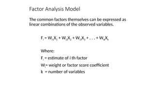
45. The common factors themselves can be expressed as
linear combinations of the observed variables.
Fi = Wi1X1 + Wi2X2 + Wi3X3 + . . . + WikXk
Where:
Fi = estimate of i th factor
Wi= weight or factor score coefficient
k = number of variables
Factor Analysis Model

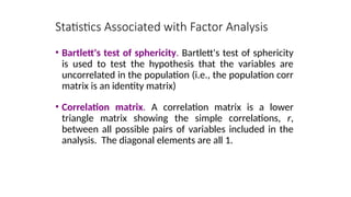
46. Statistics Associated with Factor Analysis
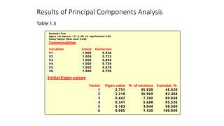
• Bartlett's test of sphericity. Bartlett's test of sphericity
is used to test the hypothesis that the variables are
uncorrelated in the population (i.e., the population corr
matrix is an identity matrix)
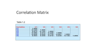
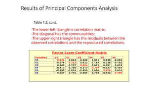
• Correlation matrix. A correlation matrix is a lower
triangle matrix showing the simple correlations, r,
between all possible pairs of variables included in the
analysis. The diagonal elements are all 1.

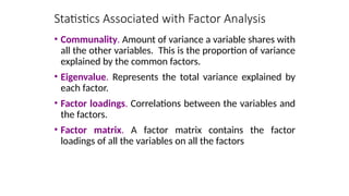
47. • Communality. Amount of variance a variable shares with
all the other variables. This is the proportion of variance
explained by the common factors.
• Eigenvalue. Represents the total variance explained by
each factor.
• Factor loadings. Correlations between the variables and
the factors.
• Factor matrix. A factor matrix contains the factor
loadings of all the variables on all the factors
Statistics Associated with Factor Analysis

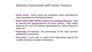
48. • Factor scores. Factor scores are composite scores estimated for
each respondent on the derived factors.
• Kaiser-Meyer-Olkin (KMO) measure of sampling adequacy. Used
to examine the appropriateness of factor analysis. High values
(between 0.5 and 1.0) indicate appropriateness. Values below 0.5
imply not.
• Percentage of variance. The percentage of the total variance
attributed to each factor.
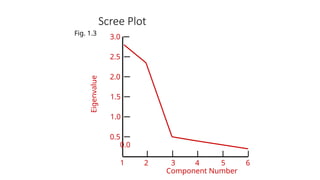
• Scree plot. A scree plot is a plot of the Eigenvalues against the
number of factors in order of extraction.
Statistics Associated with Factor Analysis

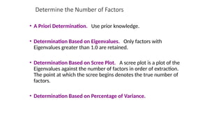
49. • A Priori Determination. Use prior knowledge.
• Determination Based on Eigenvalues. Only factors with
Eigenvalues greater than 1.0 are retained.
• Determination Based on Scree Plot. A scree plot is a plot of the
Eigenvalues against the number of factors in order of extraction.
The point at which the scree begins denotes the true number of
factors.
• Determination Based on Percentage of Variance.
Determine the Number of Factors

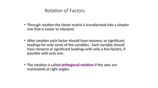
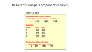
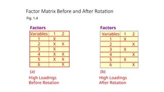
50. • Through rotation the factor matrix is transformed into a simpler
one that is easier to interpret.
• After rotation each factor should have nonzero, or significant,
loadings for only some of the variables. Each variable should
have nonzero or significant loadings with only a few factors, if
possible with only one.
• The rotation is called orthogonal rotation if the axes are
maintained at right angles.
Rotation of Factors

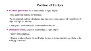
51. • Varimax procedure. Axes maintained at right angles
-Most common method for rotation.
-An orthogonal method of rotation that minimizes the number of variables with
high loadings on a factor.
-Orthogonal rotation results in uncorrelated factors.
• Oblique rotation. Axes not maintained at right angles
-Factors are correlated.
-Oblique rotation should be used when factors in the population are likely to be
strongly correlated.
Rotation of Factors

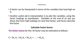
52. • A factor can be interpreted in terms of the variables that load high on
it.
• Another useful aid in interpretation is to plot the variables, using the
factor loadings as coordinates. Variables at the end of an axis are
those that have high loadings on only that factor, and hence describe
the factor.
Calculate Factor Scores
The factor scores for the i th factor may be estimated as follows:
Fi = Wi1 X1 + Wi2 X2 + Wi3 X3 + . . . + Wik Xk
Interpret Factors

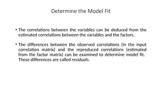
53. • The correlations between the variables can be deduced from the
estimated correlations between the variables and the factors.
• The differences between the observed correlations (in the input
correlation matrix) and the reproduced correlations (estimated
from the factor matrix) can be examined to determine model fit.
These differences are called residuals.
Determine the Model Fit

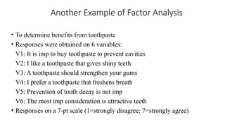
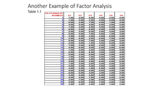
54. Another Example of Factor Analysis
• To determine benefits from toothpaste
• Responses were obtained on 6 variables:
V1: It is imp to buy toothpaste to prevent cavities
V2: I like a toothpaste that gives shiny teeth
V3: A toothpaste should strengthen your gums
V4: I prefer a toothpaste that freshens breath
V5: Prevention of tooth decay is not imp
V6: The most imp consideration is attractive teeth
• Responses on a 7-pt scale (1=strongly disagree; 7=strongly agree)

55. Another Example of Factor Analysis
RE S PONDE NT
NUMBE R V1 V2 V3 V4 V5 V6
1 7.00 3.00 6.00 4.00 2.00 4.00
2 1.00 3.00 2.00 4.00 5.00 4.00
3 6.00 2.00 7.00 4.00 1.00 3.00
4 4.00 5.00 4.00 6.00 2.00 5.00
5 1.00 2.00 2.00 3.00 6.00 2.00
6 6.00 3.00 6.00 4.00 2.00 4.00
7 5.00 3.00 6.00 3.00 4.00 3.00
8 6.00 4.00 7.00 4.00 1.00 4.00
9 3.00 4.00 2.00 3.00 6.00 3.00
10 2.00 6.00 2.00 6.00 7.00 6.00
11 6.00 4.00 7.00 3.00 2.00 3.00
12 2.00 3.00 1.00 4.00 5.00 4.00
13 7.00 2.00 6.00 4.00 1.00 3.00
14 4.00 6.00 4.00 5.00 3.00 6.00
15 1.00 3.00 2.00 2.00 6.00 4.00
16 6.00 4.00 6.00 3.00 3.00 4.00
17 5.00 3.00 6.00 3.00 3.00 4.00
18 7.00 3.00 7.00 4.00 1.00 4.00
19 2.00 4.00 3.00 3.00 6.00 3.00
20 3.00 5.00 3.00 6.00 4.00 6.00
21 1.00 3.00 2.00 3.00 5.00 3.00
22 5.00 4.00 5.00 4.00 2.00 4.00
23 2.00 2.00 1.00 5.00 4.00 4.00
24 4.00 6.00 4.00 6.00 4.00 7.00
25 6.00 5.00 4.00 2.00 1.00 4.00
26 3.00 5.00 4.00 6.00 4.00 7.00
27 4.00 4.00 7.00 2.00 2.00 5.00
28 3.00 7.00 2.00 6.00 4.00 3.00
29 4.00 6.00 3.00 7.00 2.00 7.00
30 2.00 3.00 2.00 4.00 7.00 2.00
Table 1.1

56. Correlation Matrix
Variables V1 V2 V3 V4 V5 V6
V1 1.000
V2 - 0.530 1.000
V3 0.873 - 0.155 1.000
V4 - 0.086 0.572 - 0.248 1.000
V5 - 0.858 0.020 - 0.778 - 0.007 1.000
V6 0.004 0.640 - 0.018 0.640 - 0.136 1.000
Table 1.2

57. Results of Principal Components Analysis
Bartlett’s Test
Apprx. chi-square= 111.3, df= 15, significance= 0.00
Kaiser-Meyer-Olkin msa= 0.660
Communalities
Variables Initial Extraction
V1 1.000 0.926
V2 1.000 0.723
V3 1.000 0.894
V4 1.000 0.739
V5 1.000 0.878
V6 1.000 0.790
Initial Eigen values
Factor Eigen value % of variance Cumulat. %
1 2.731 45.520 45.520
2 2.218 36.969 82.488
3 0.442 7.360 89.848
4 0.341 5.688 95.536
5 0.183 3.044 98.580
6 0.085 1.420 100.000
Table 1.3

58. Results of Principal Components Analysis
Extraction Sums of Squared Loadings
Factor Eigen value % of variance Cumulat. %
1 2.731 45.520 45.520
2 2.218 36.969 82.488
Factor Matrix
Variables Factor 1 Factor 2
V1 0.928 0.253
V2 -0.301 0.795
V3 0.936 0.131
V4 -0.342 0.789
V5 -0.869 -0.351
V6 -0.177 0.871
Rotation Sums of Squared Loadings
Factor Eigenvalue % of variance Cumulat. %
1 2.688 44.802 44.802
2 2.261 37.687 82.488
Table 1.3, cont.

59. Results of Principal Components Analysis
Rotated Factor Matrix
Variables Factor 1 Factor 2
V1 0.962 -0.027
V2 -0.057 0.848
V3 0.934 -0.146
V4 -0.098 0.845
V5 -0.933 -0.084
V6 0.083 0.885
Factor Score Coefficient Matrix
Variables Factor 1 Factor 2
V1 0.358 0.011
V2 -0.001 0.375
V3 0.345 -0.043
V4 -0.017 0.377
V5 -0.350 -0.059
V6 0.052 0.395
Table 1.3, cont.

60. Factor Score Coefficient Matrix
Variables V1 V2 V3 V4 V5 V6
V1 0.926 0.024 -0.029 0.031 0.038 -0.053
V2 -0.078 0.723 0.022 -0.158 0.038 -0.105
V3 0.902 -0.177 0.894 -0.031 0.081 0.033
V4 -0.117 0.730 -0.217 0.739 -0.027 -0.107
V5 -0.895 -0.018 -0.859 0.020 0.878 0.016
V6 0.057 0.746 -0.051 0.748 -0.152 0.790
-The lower-left triangle is correlation matrix;
-The diagonal has the communalities;
-The upper-right triangle has the residuals between the
observed correlations and the reproduced correlations.
Results of Principal Components Analysis
Table 1.3, cont.

61. Scree Plot
0.5
2 5
4
3 6
Component Number
0.0
2.0
3.0
Eigenvalue
1.0
1.5
2.5
1
Fig. 1.3

62. Factor Matrix Before and After Rotation
Factors
(a)
High Loadings
Before Rotation
Fig. 1.4
(b)
High Loadings
After Rotation
Factors
Variables
1
2
3
4
5
6
1
X
X
X
X
X
2
X
X
X
X
1
X
X
X
2
X
X
X
Variables
1
2
3
4
5
6