Downloaded 636 times

1. The document discusses time response analysis of systems using poles and zeros. It describes different types of system responses including first-order, second-order, and higher-order systems. 2. Key aspects covered include the relationship between poles/zeros and forced/natural responses, effects of varying damping ratios, and specifications for step responses including rise time and settling time. 3. Various figures and examples illustrate pole-zero placement and resulting step responses for different system orders and damping scenarios.
Introduction to Chapter 4 focusing on time response in various control systems.
Discusses forced and natural responses, and how poles and zeros facilitate system response analysis.
Describes poles as values making transfer functions infinite, connecting denominator roots with numerator roots.
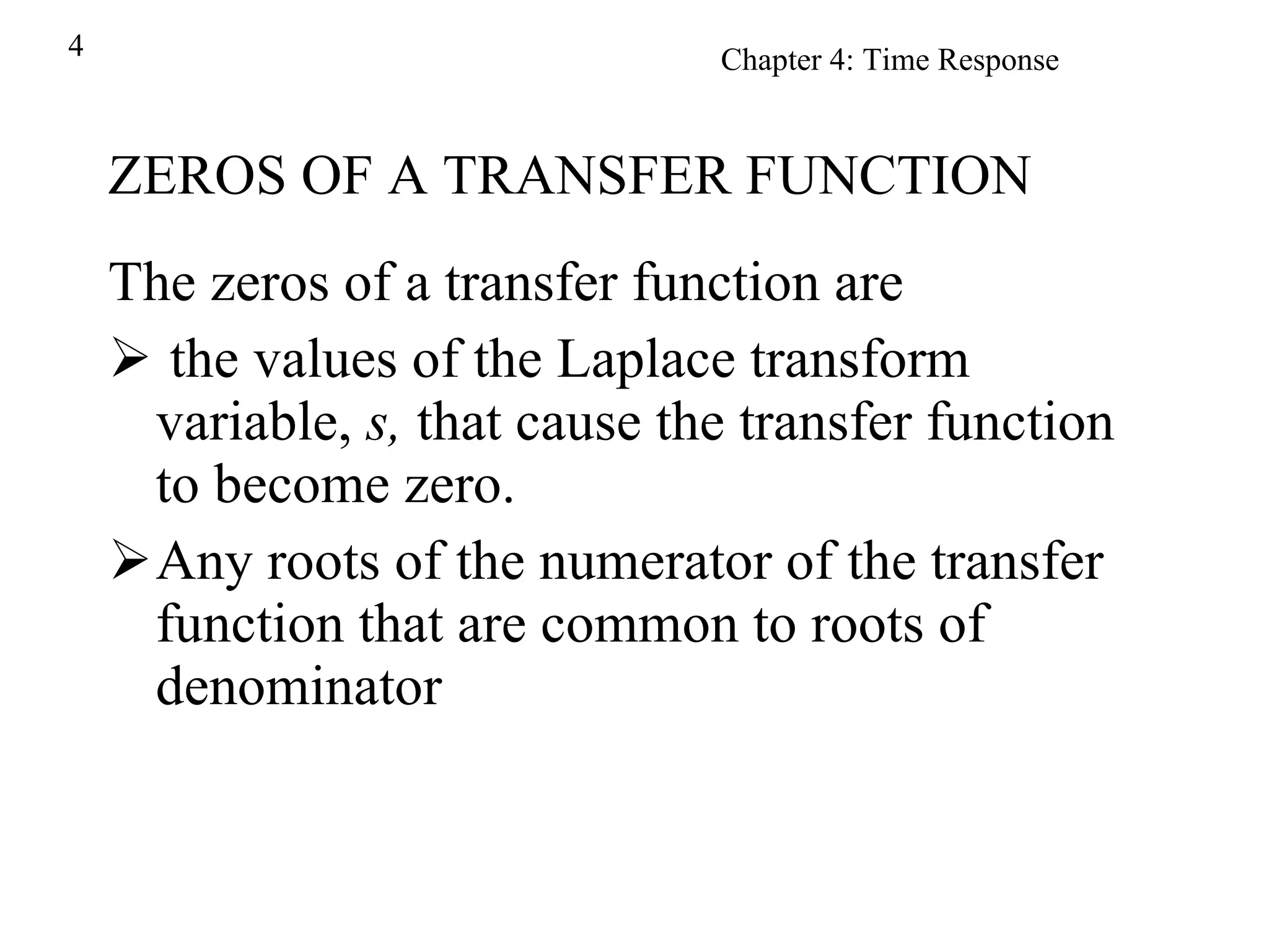
Zeros are explained as values causing the transfer function to be zero, related to numerator roots.
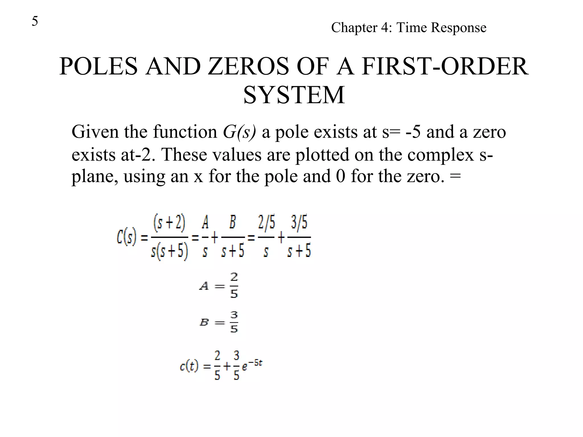
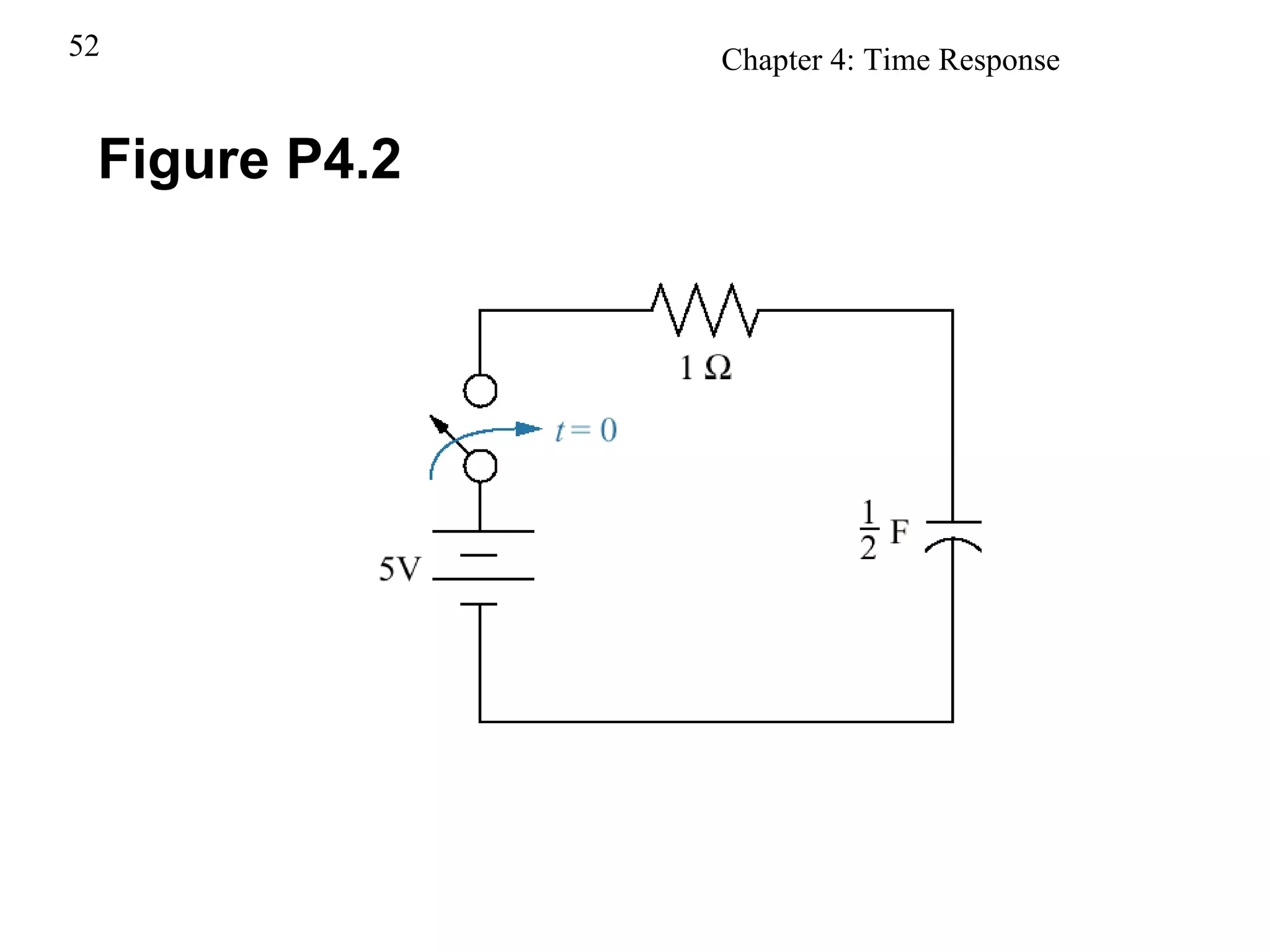
Analyzes a first-order system with a specified pole at s=-5 and zero at s=-2, with visual representation.
Identifies the roles of poles and zeros in generating forced and natural responses, emphasizing exponential forms.
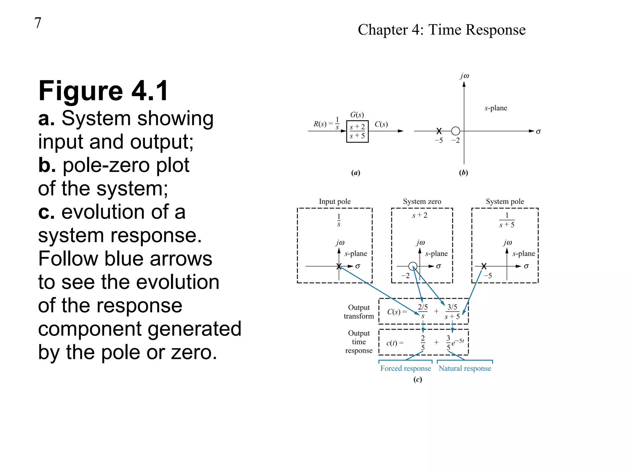
Figures illustrating system response evolution through input and output mappings and pole-zero plots.
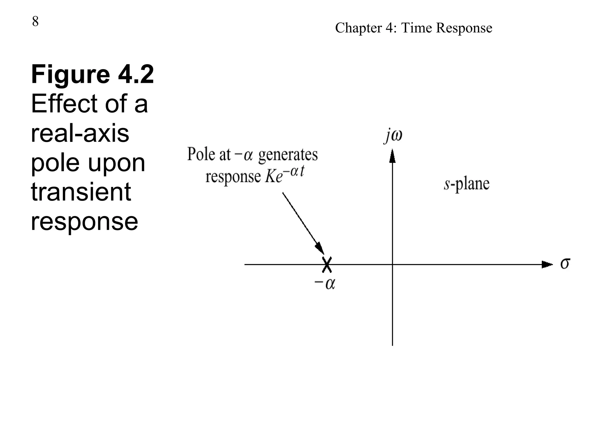
Demonstrates how a real-axis pole influences the transient response of a system.
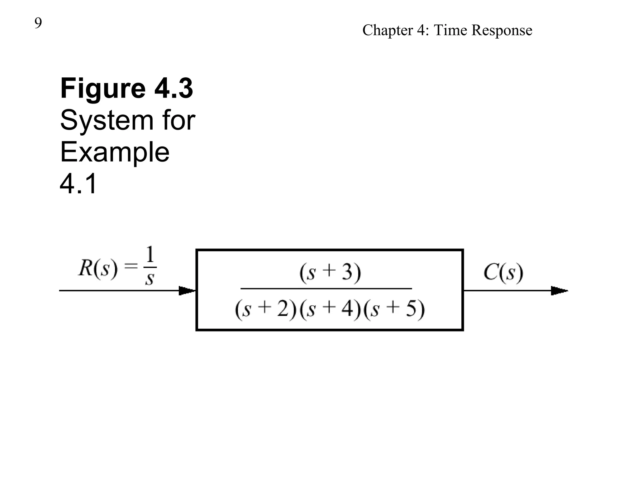
Visual representation of a specific system used for analysis in the presentation.
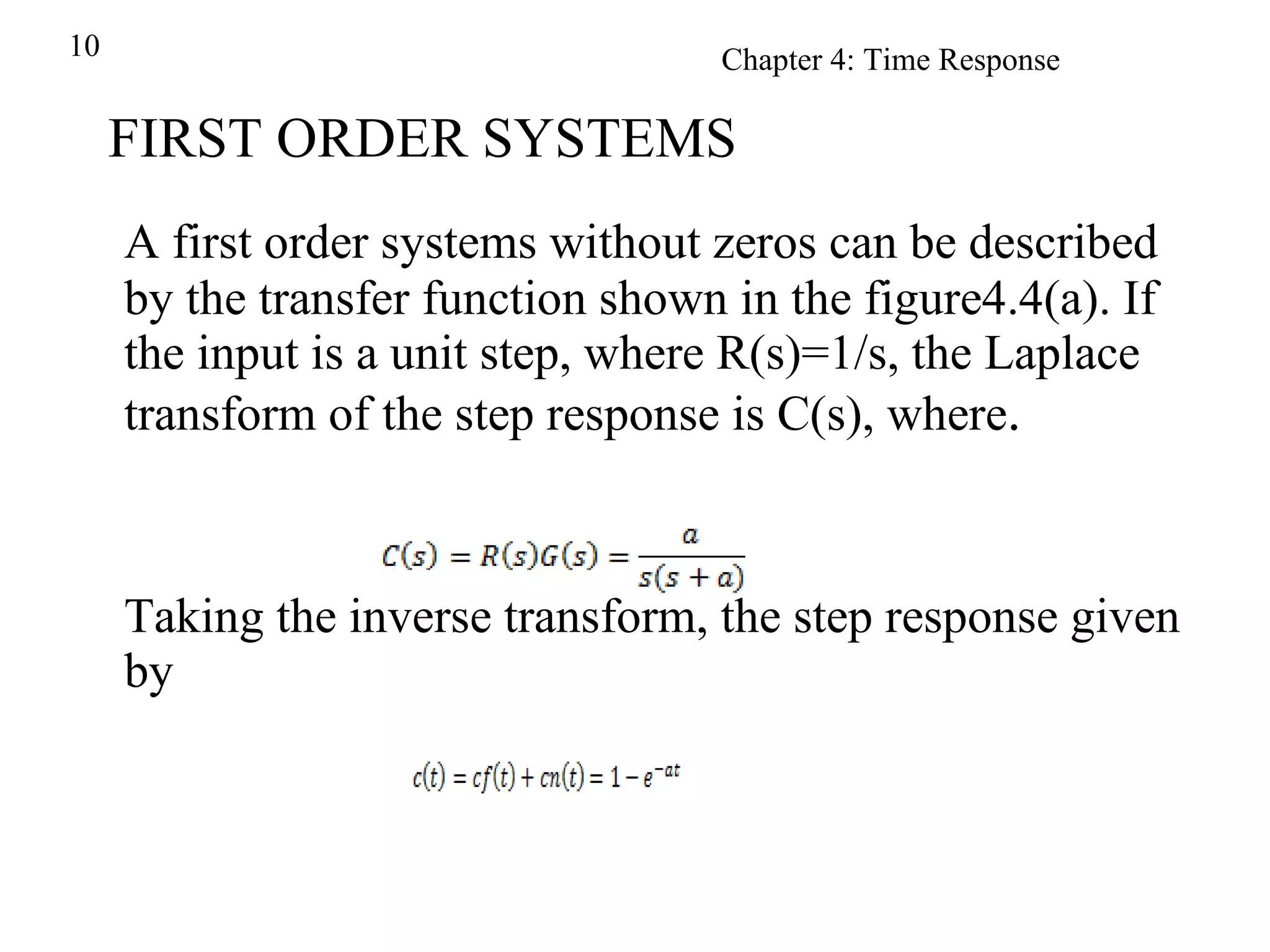
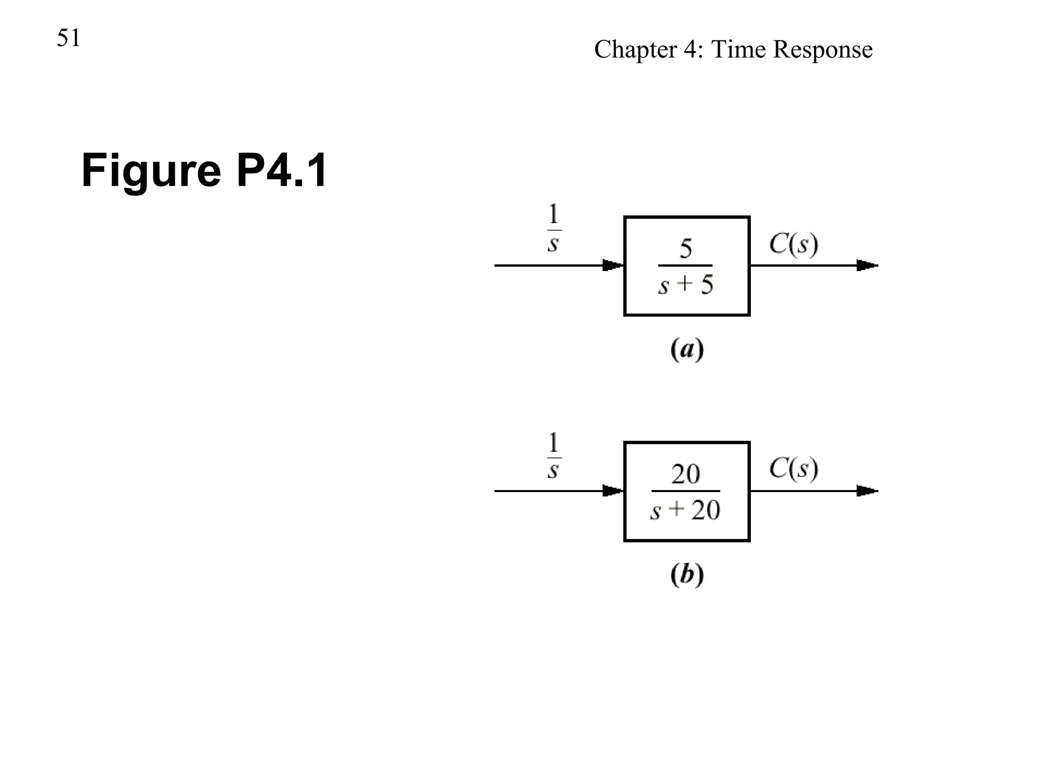
Details of first-order systems without zeros, with unit step input responses elaborated.
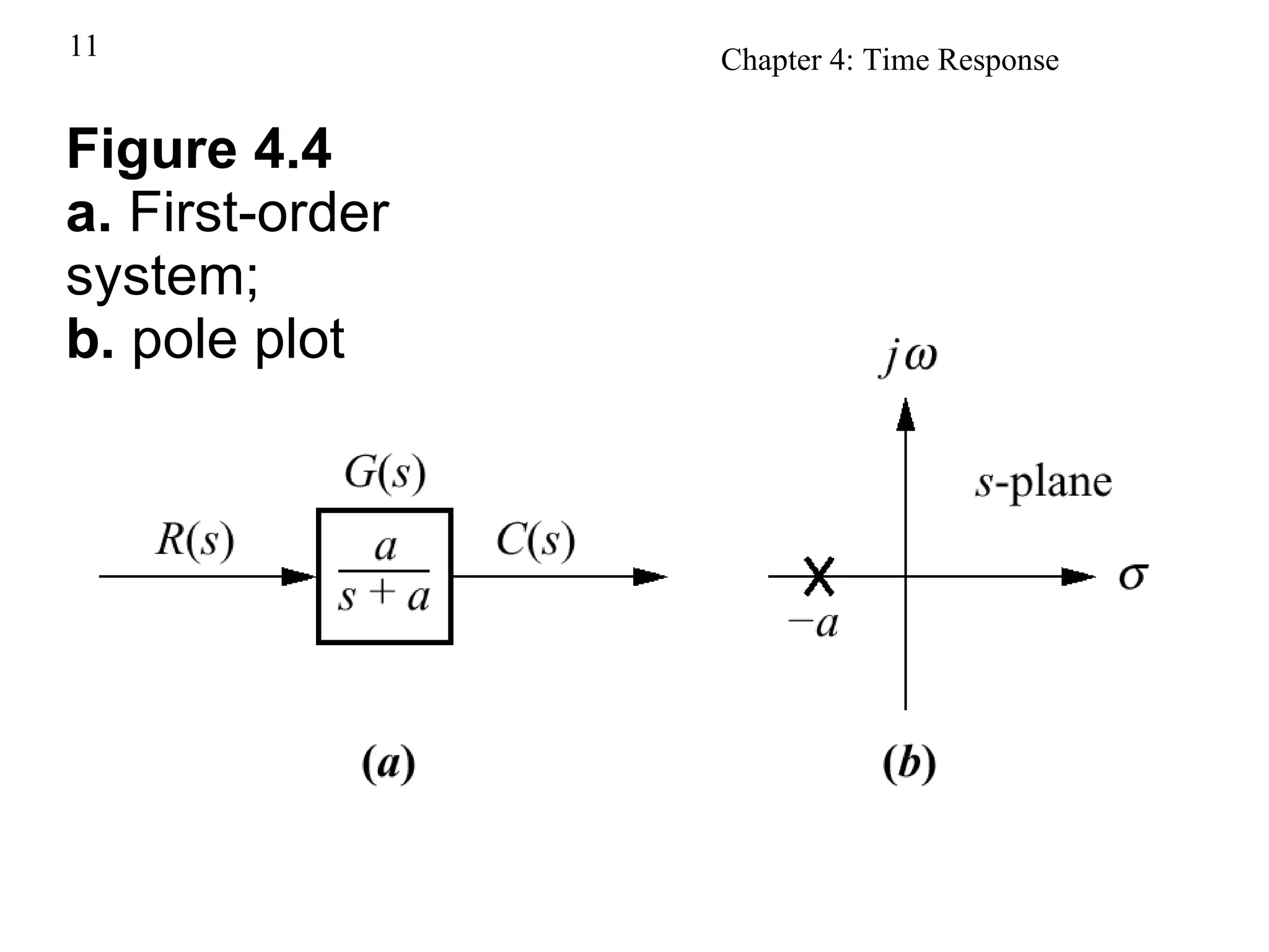
Pole plot and graphical illustrations of first-order system behaviors.
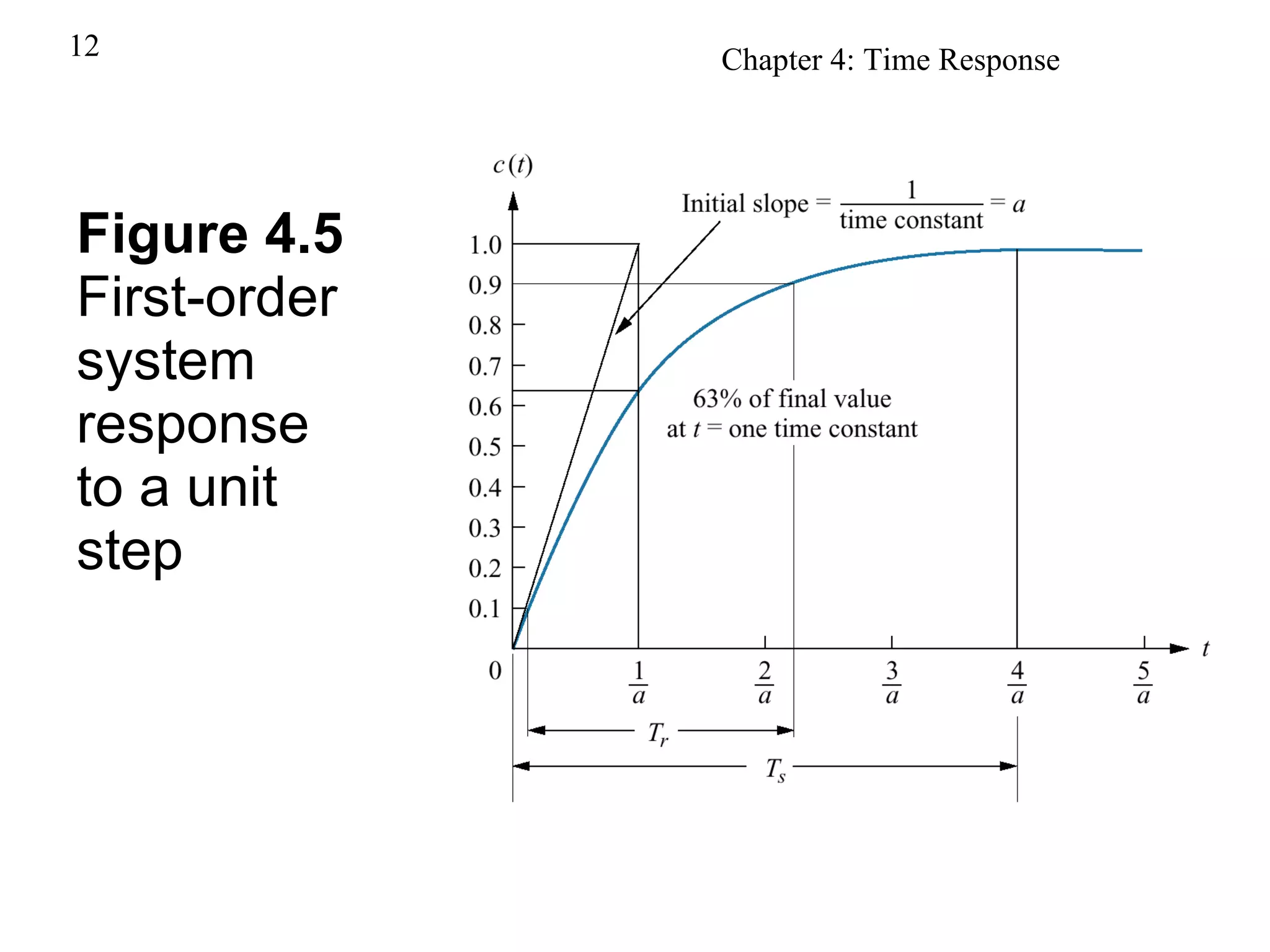
Graphical representation of a first-order system's response to a unit step input.
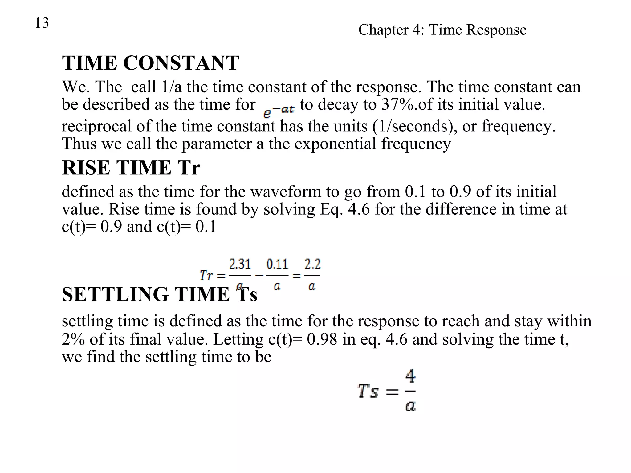
Explains time constant definitions and measurements such as rise time and settling time.
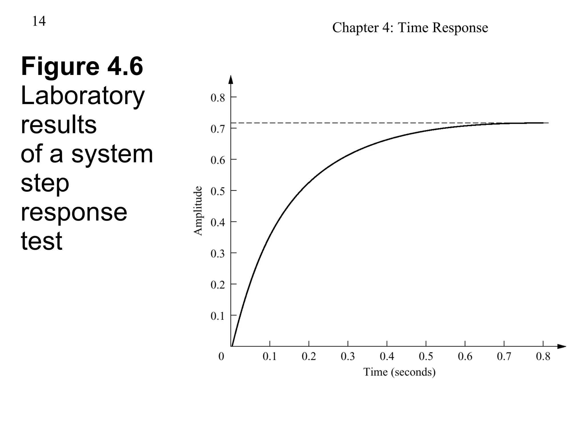
Presentation of laboratory results showcasing system step response tests.
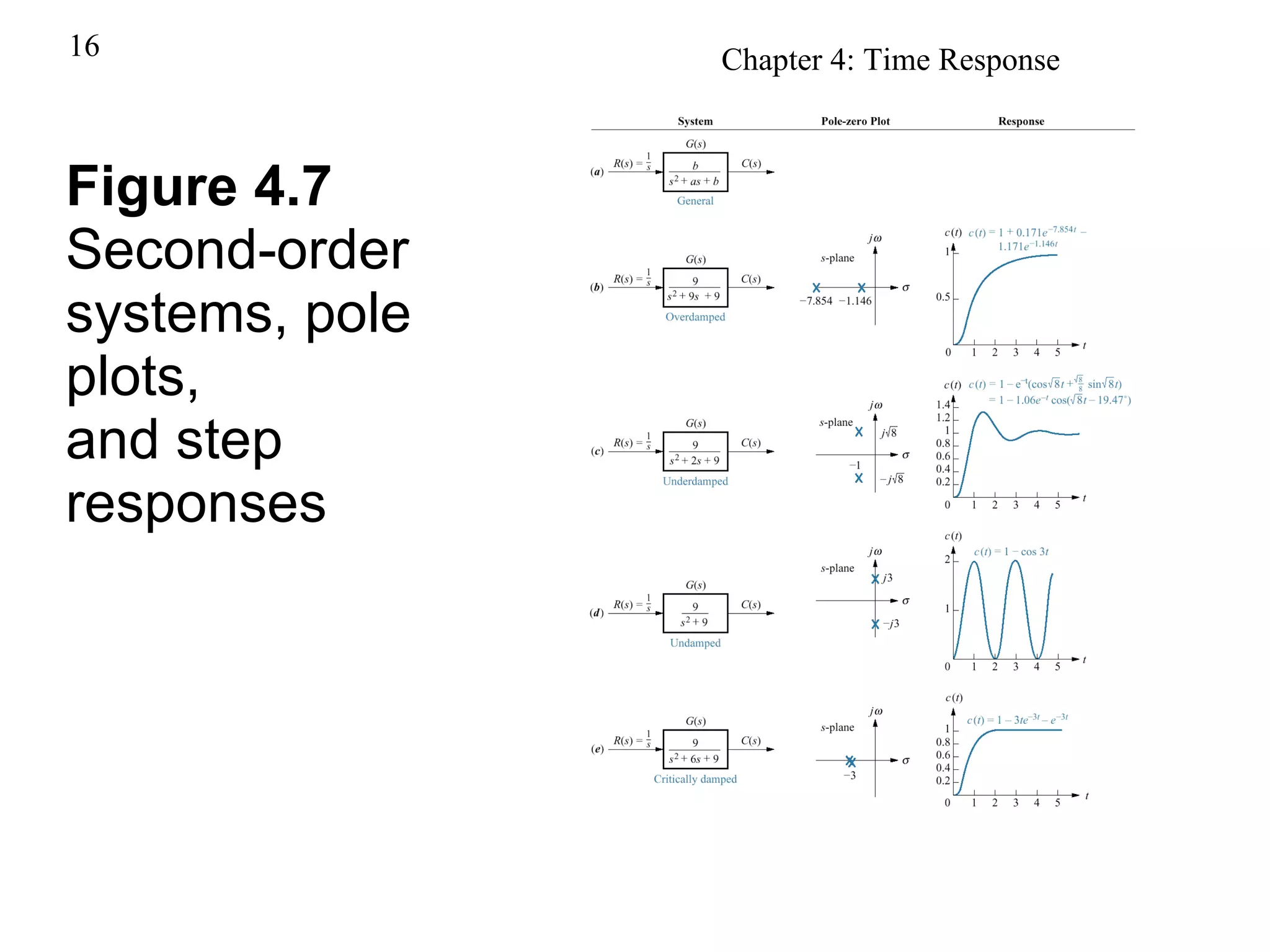
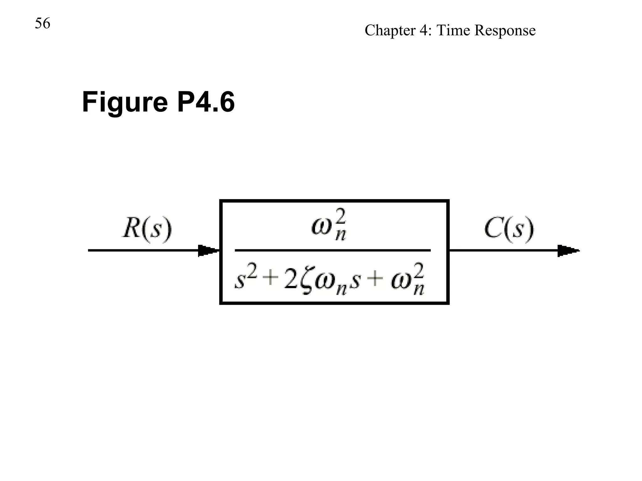
Examines second-order systems, highlighting how parameters affect diverse response types.
Figures illustrating second-order systems, pole plots, and varied step responses.
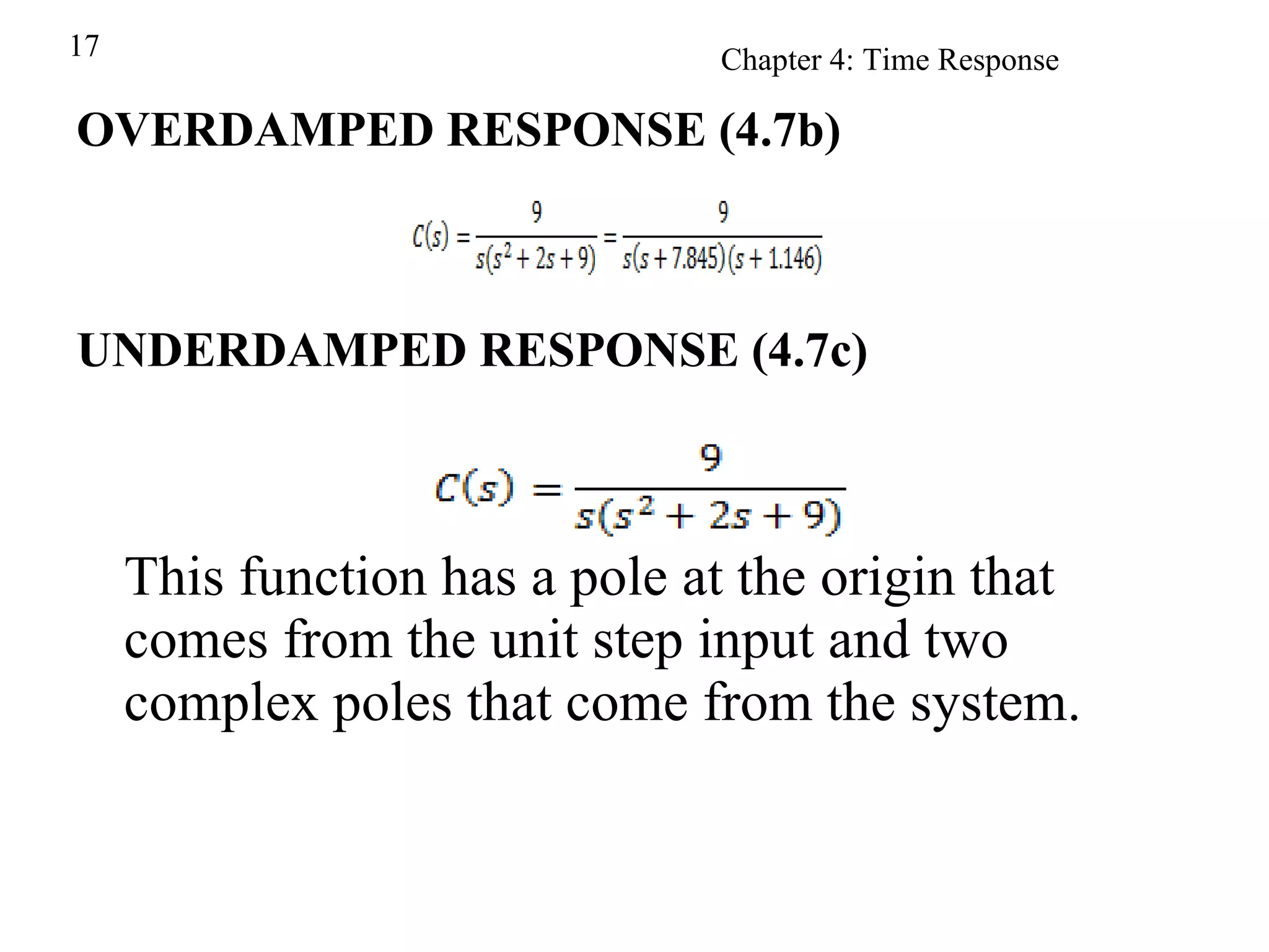
Description of system responses: overdamped, underdamped, and their poles' implications.
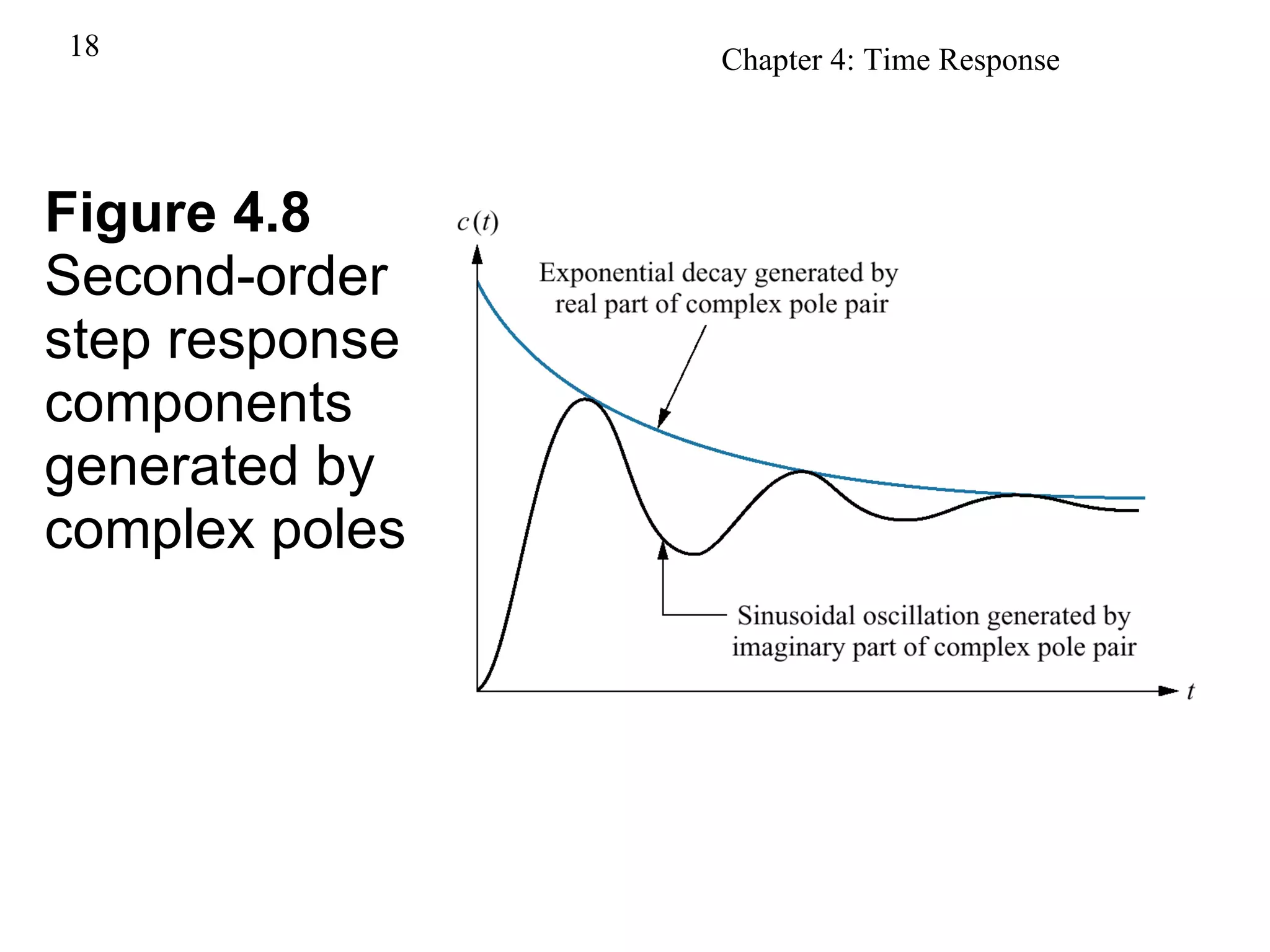
Visual representation of components generated by complex poles in a second-order system.
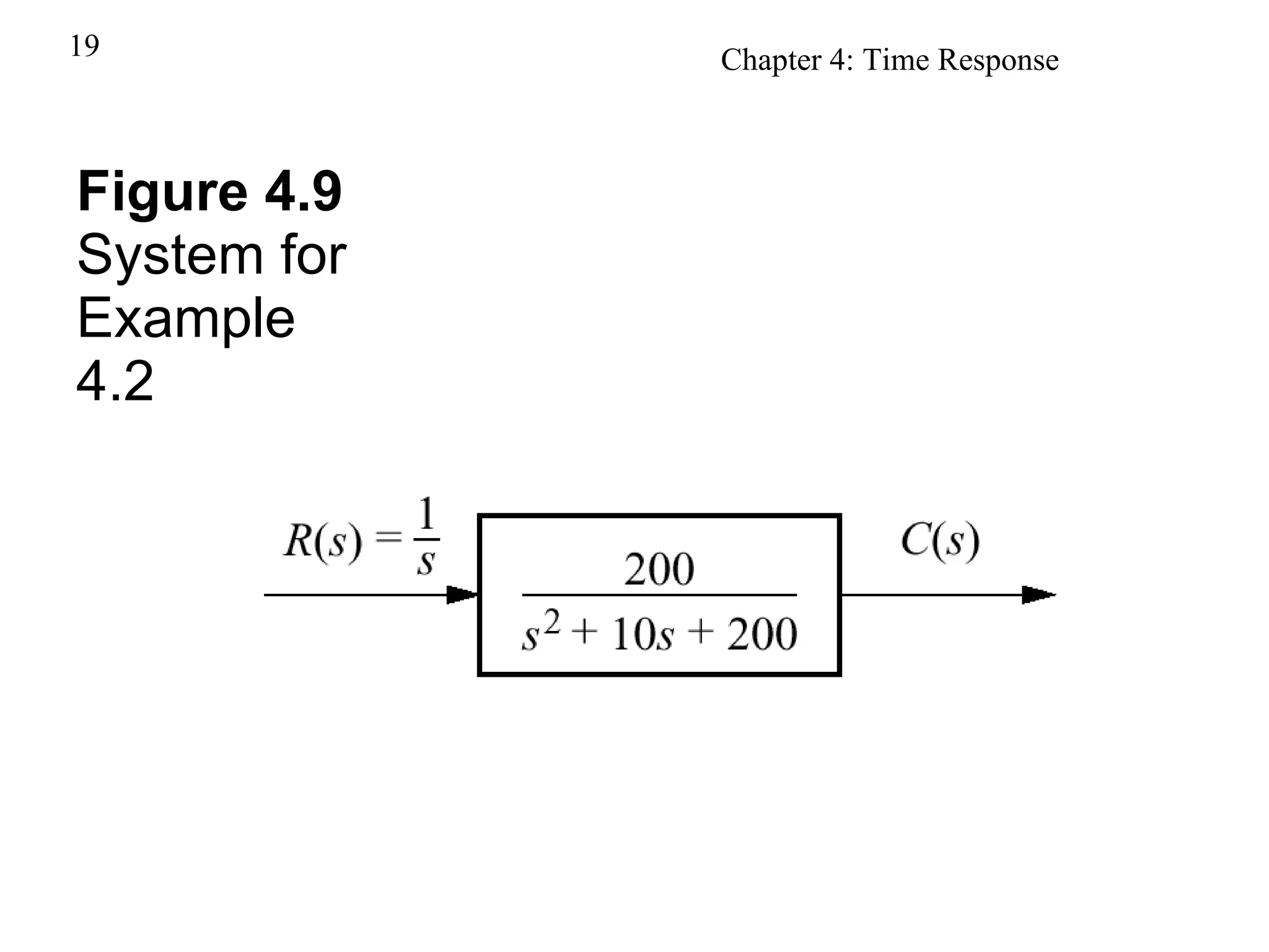
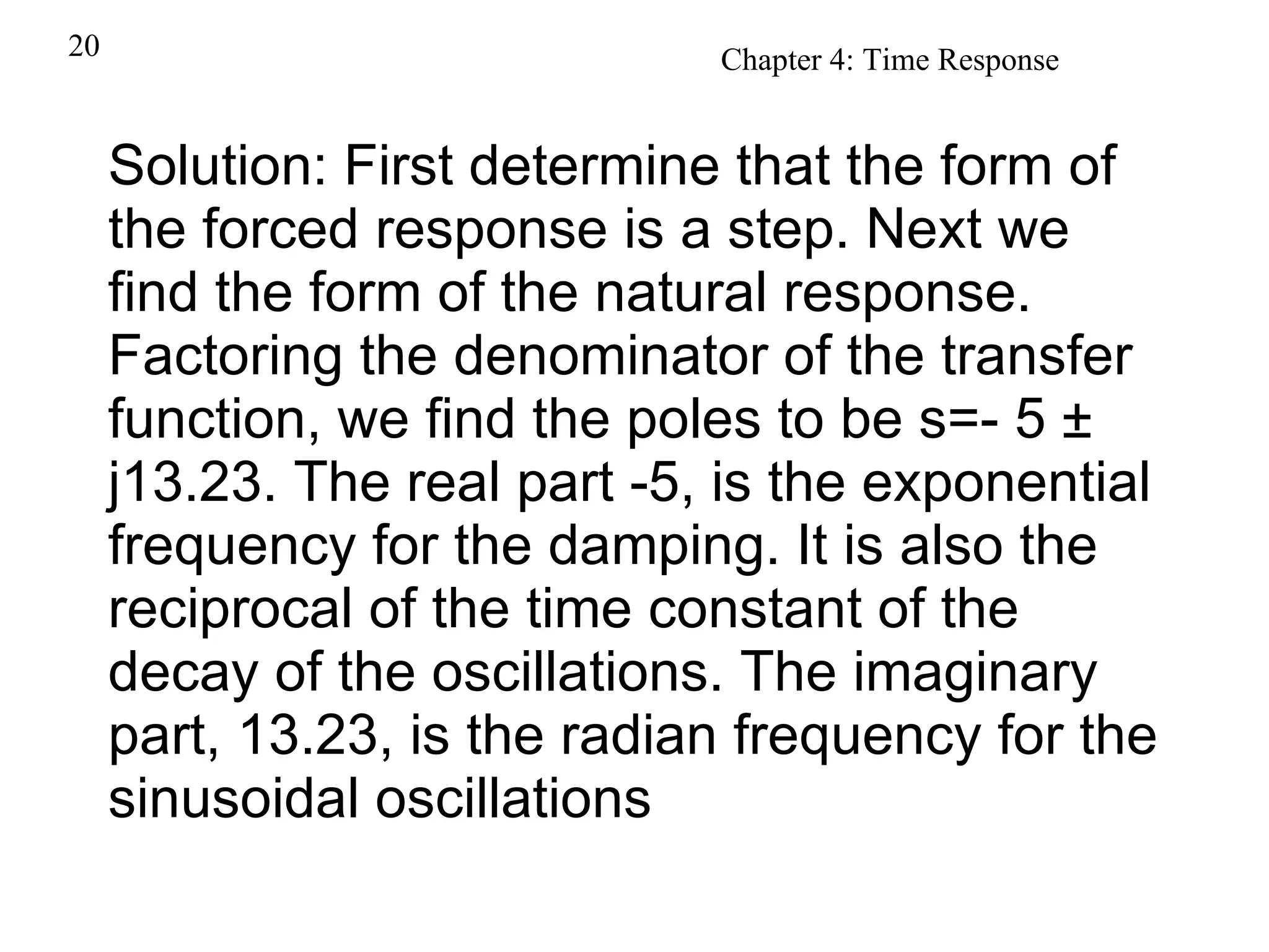
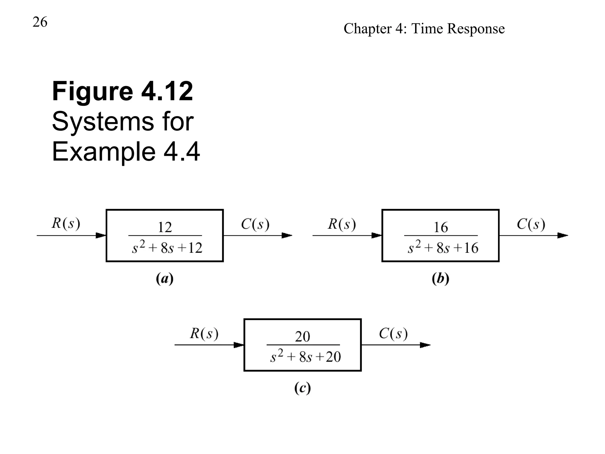
Detailed example of determining poles for a second-order system analysis.
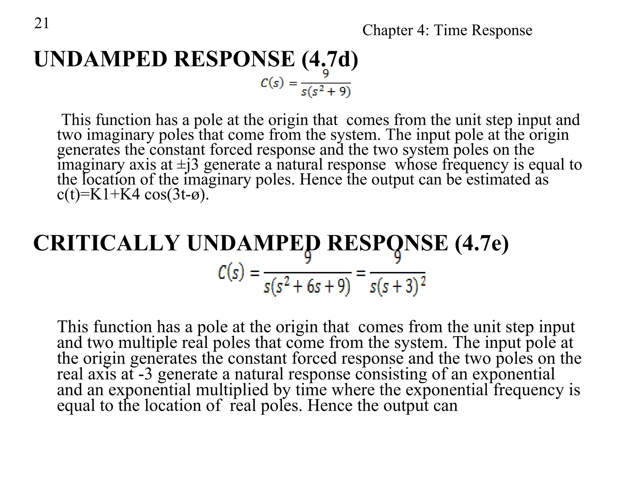
Explanation of undamped responses from a system with imaginary poles, showcasing output characteristics.
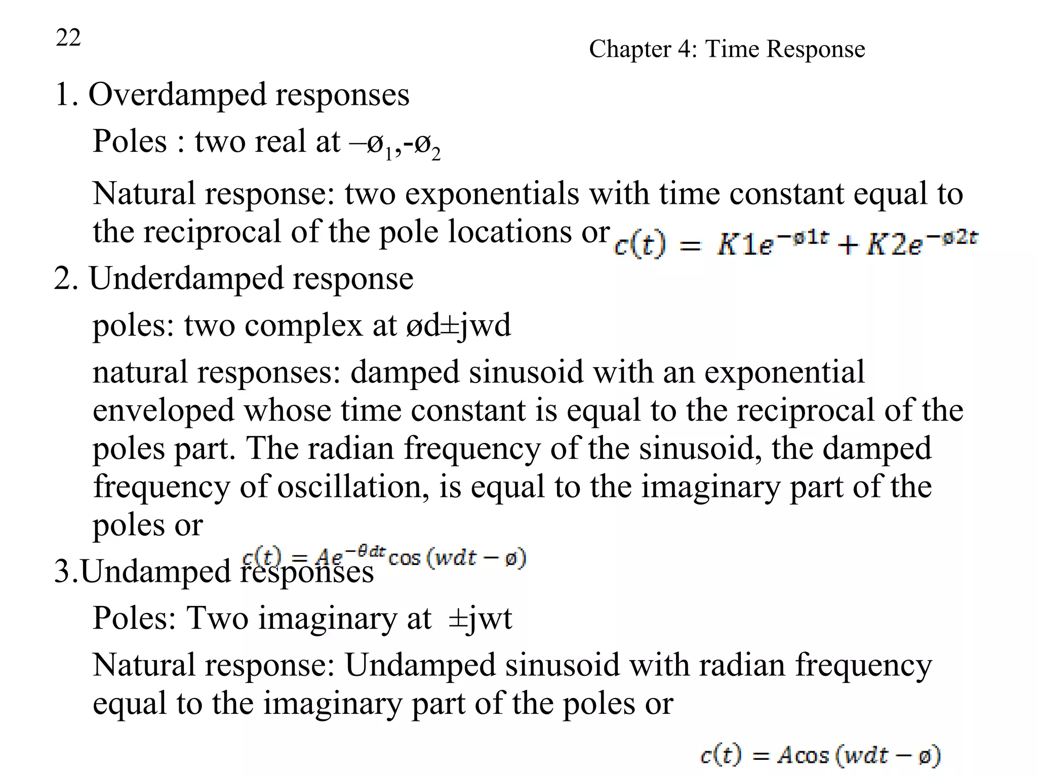
Comparison of overdamped, underdamped, and undamped response characteristics based on pole locations.
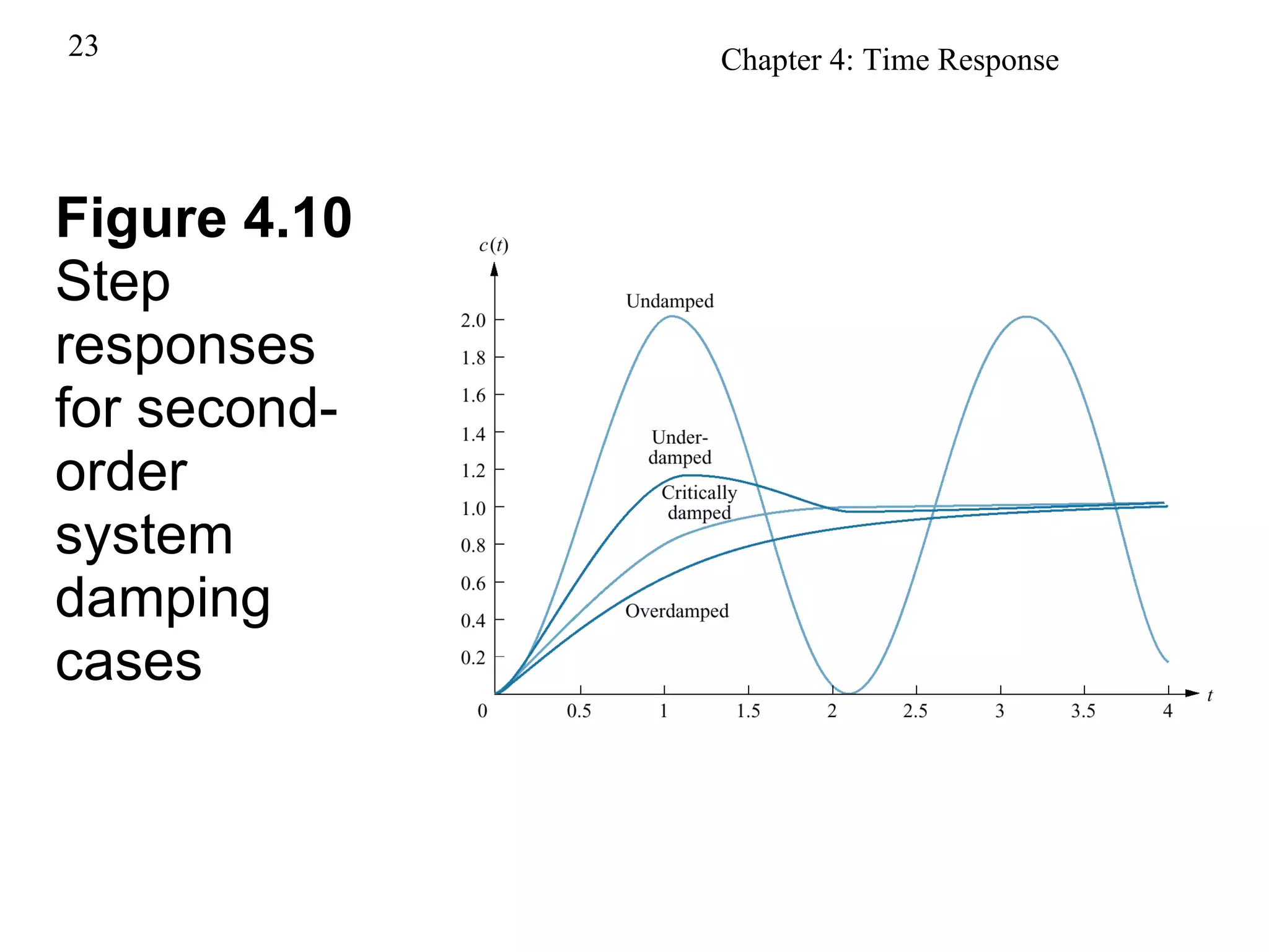
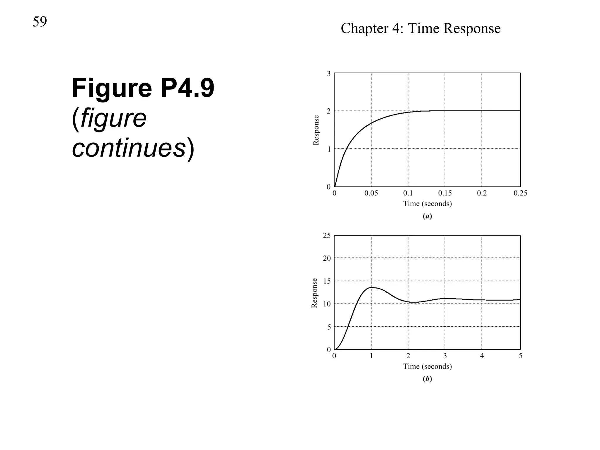
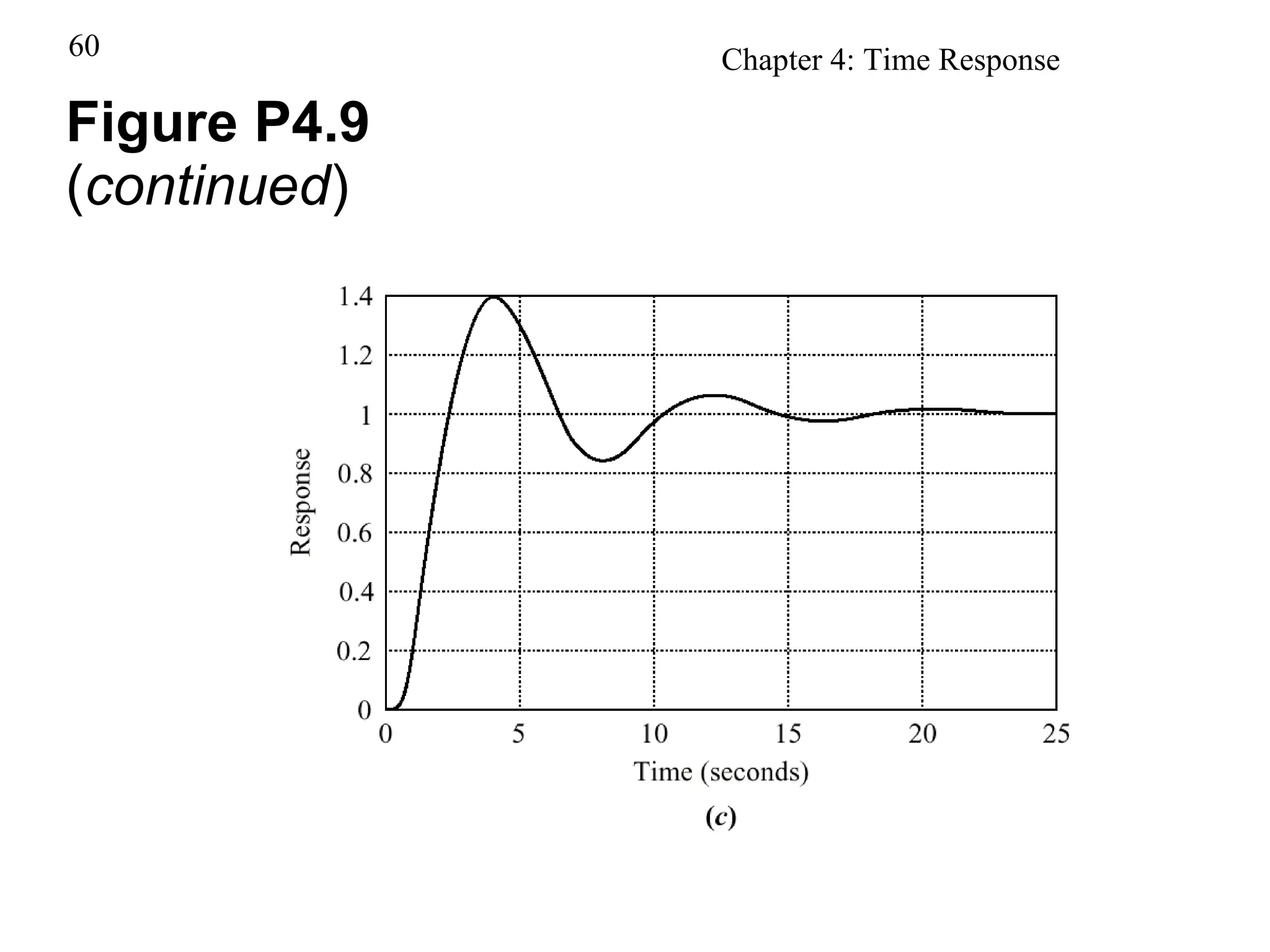
Presentation of step responses for various second-order system damping cases.
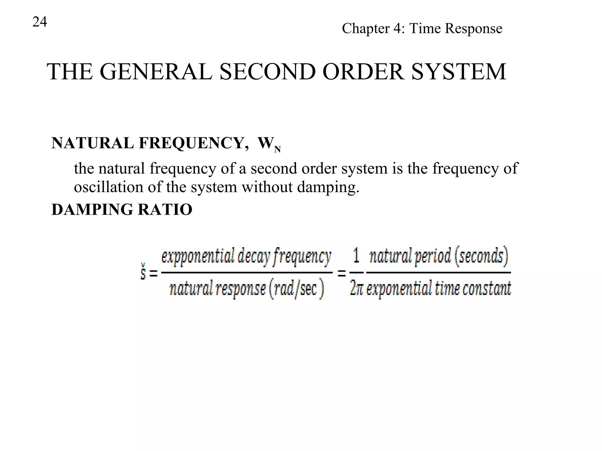
Introduction to natural frequency and the role of damping ratio in second-order systems.
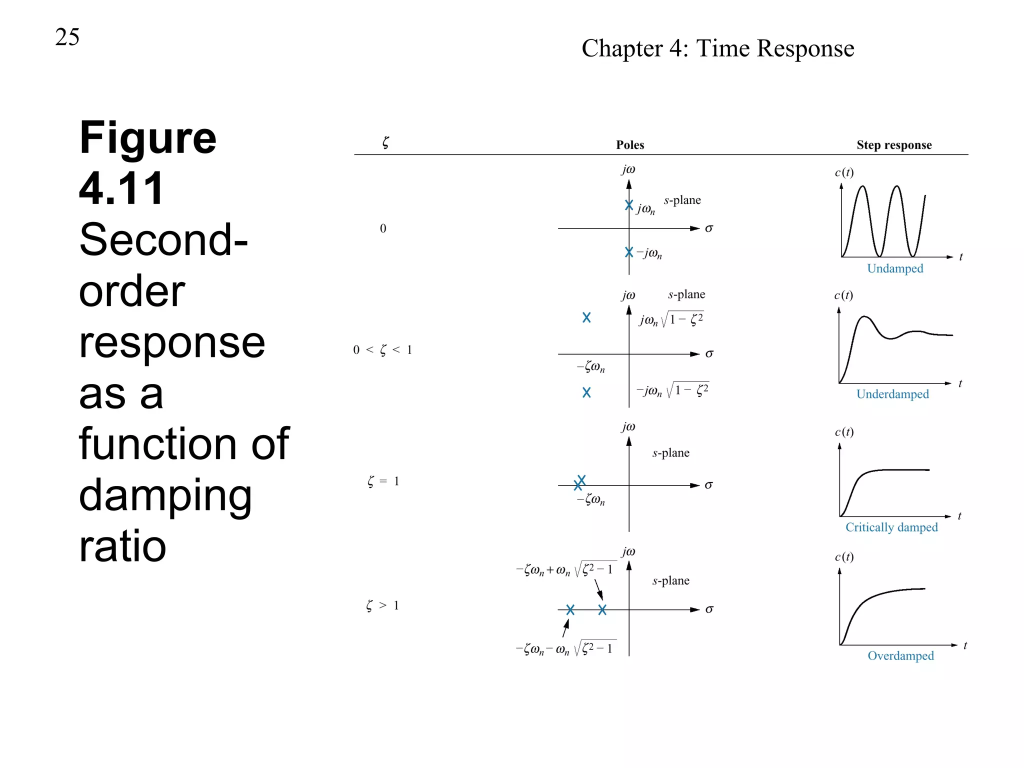
Visualizing how varying damping ratios affect the second-order system responses.
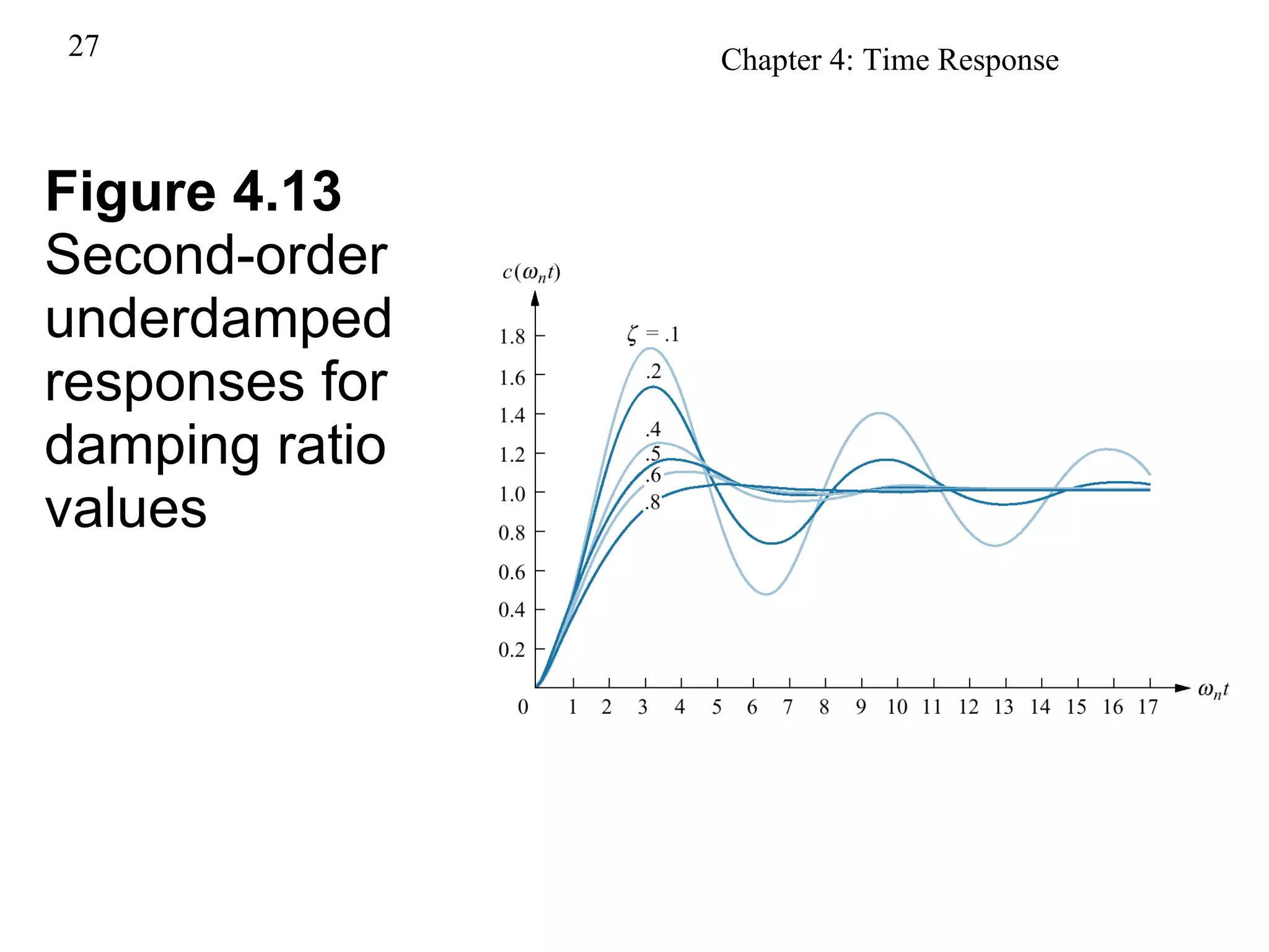
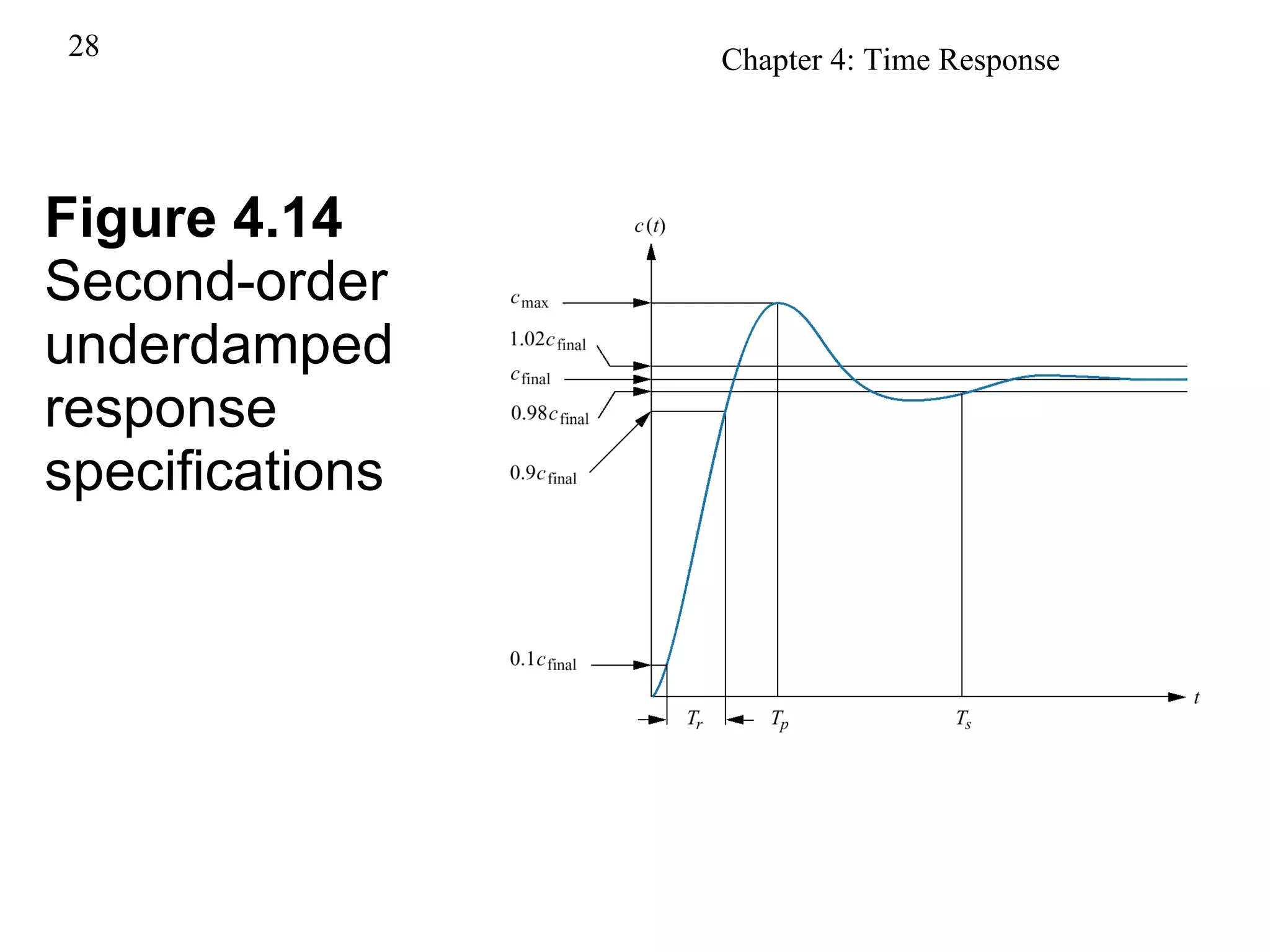
Explores underdamped responses and specification variations as damping ratios change.
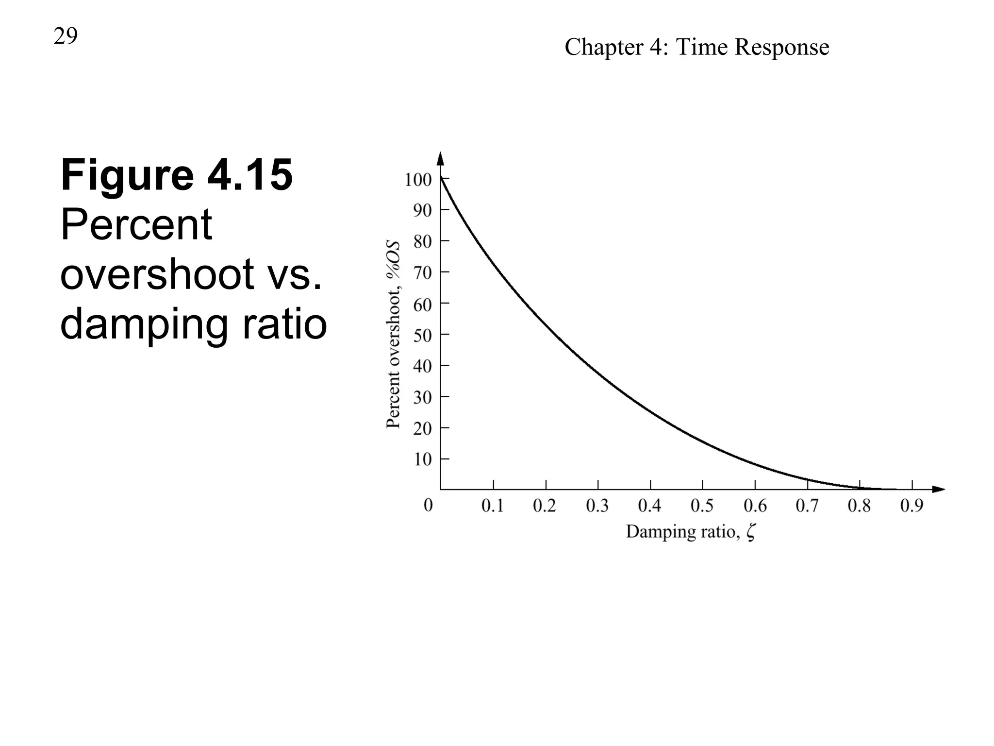
Analyzes percent overshoot related to changing damping ratio values in second-order systems.
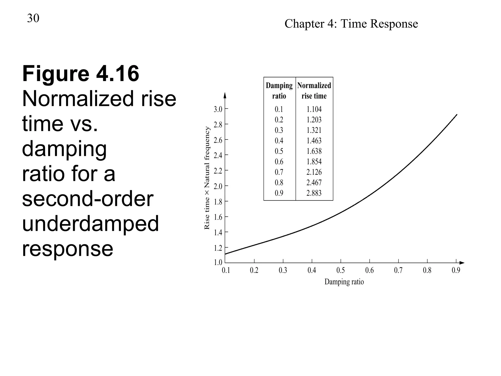
Illustrates normalized rise time vs damping ratio for second-order underdamped responses.
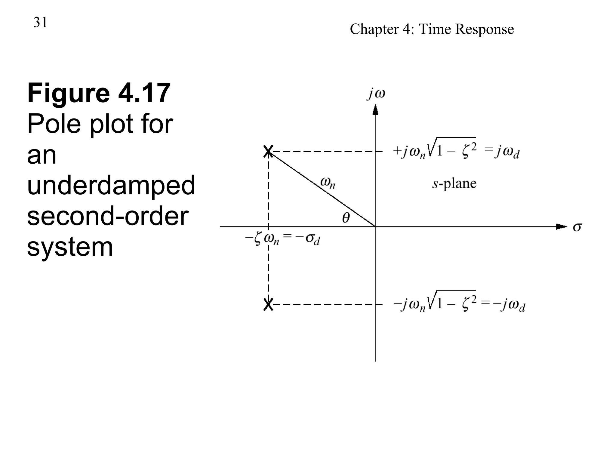
Displays pole plots showcasing underdamped second-order system characteristics.
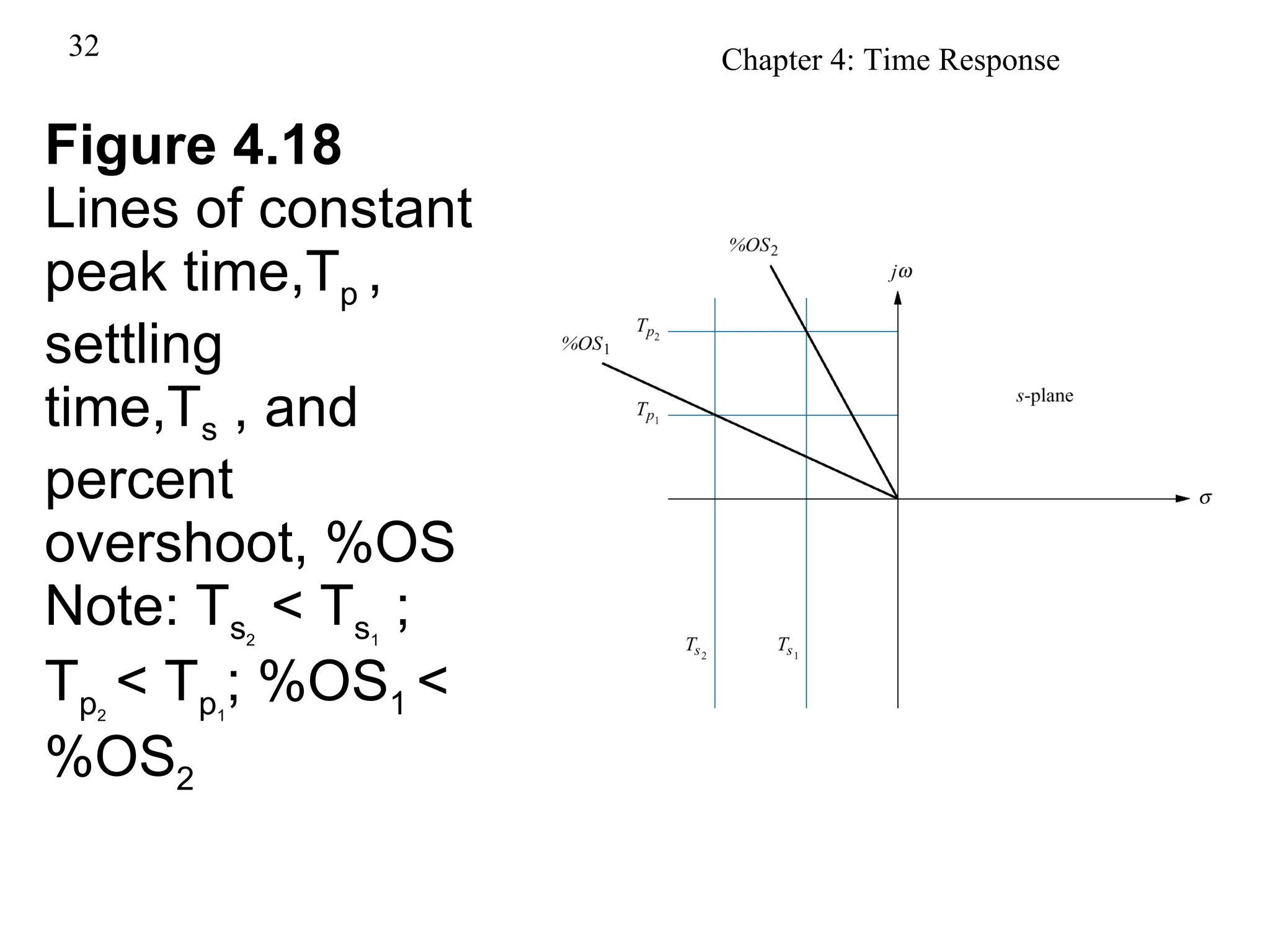
Introduces timing metrics like peak time, settling time, and their relationship to damping ratio.
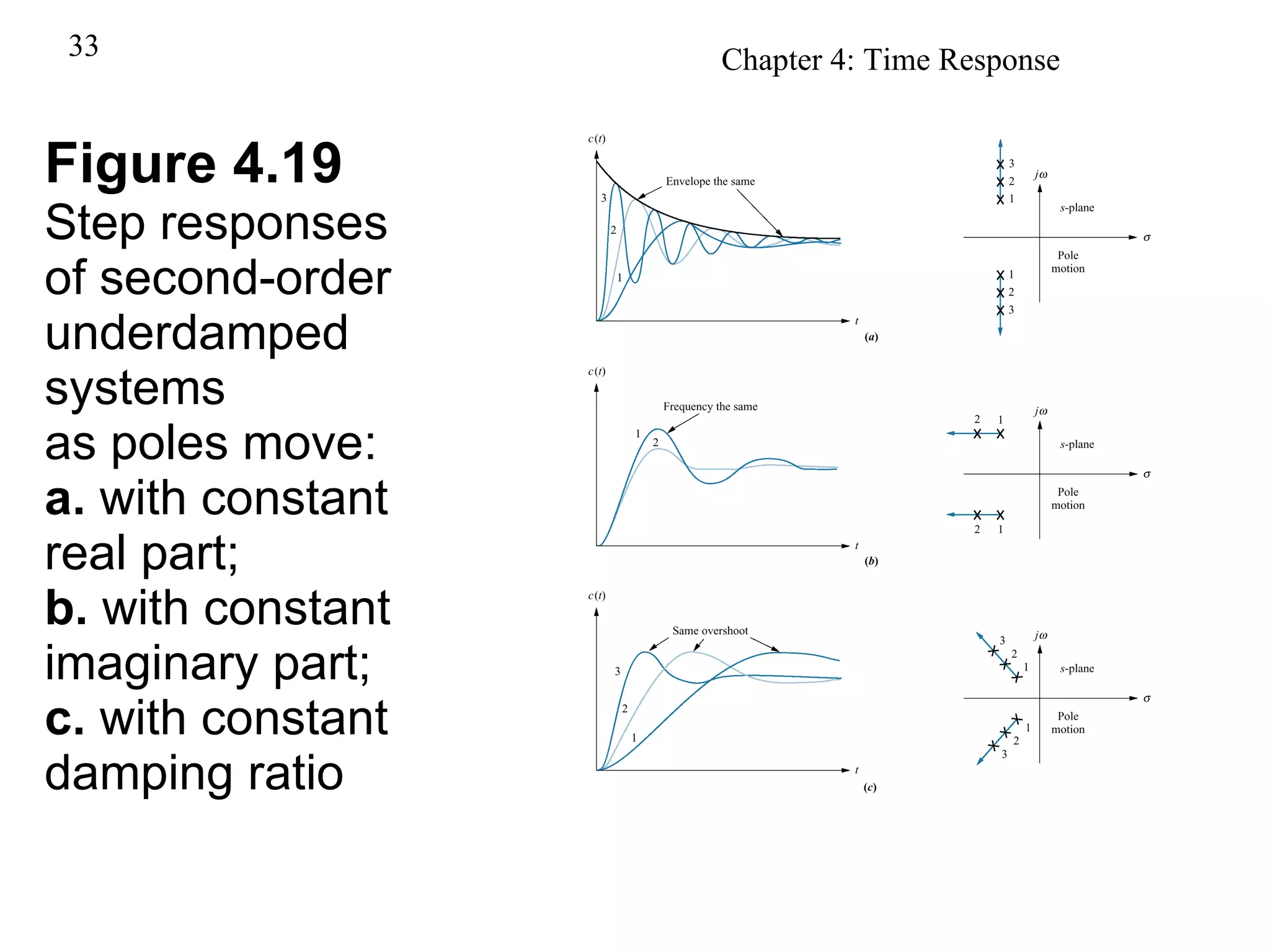
Variations in step responses as poles of second-order underdamped systems move.
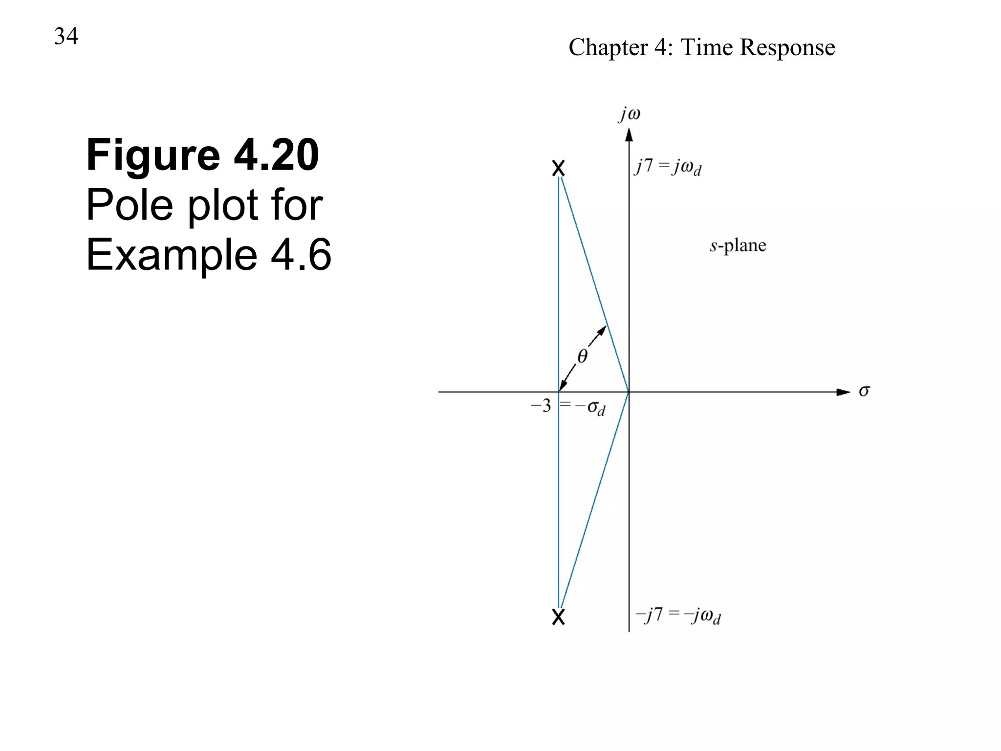
Detailed representation of pole plot for specific example provided.
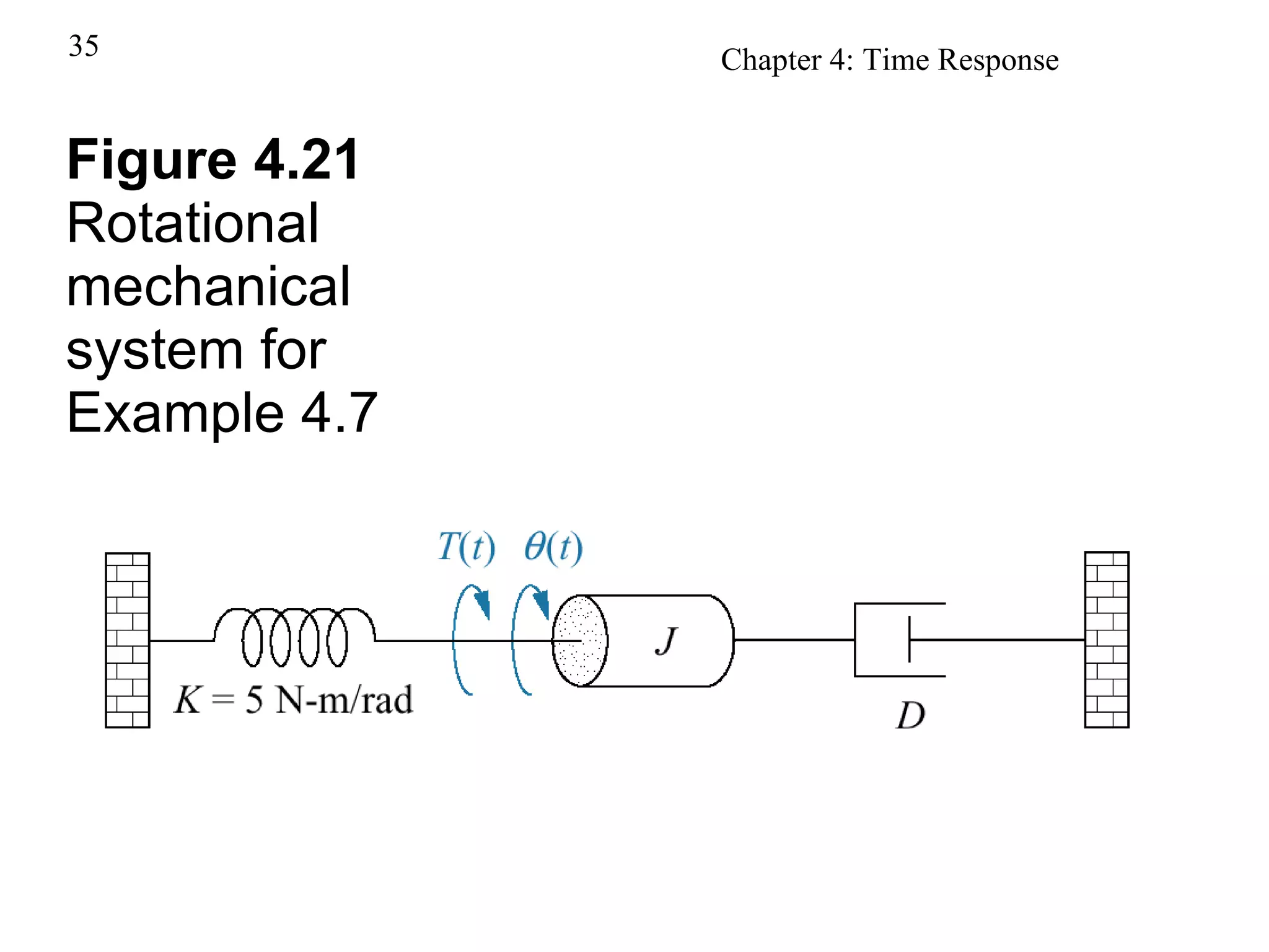
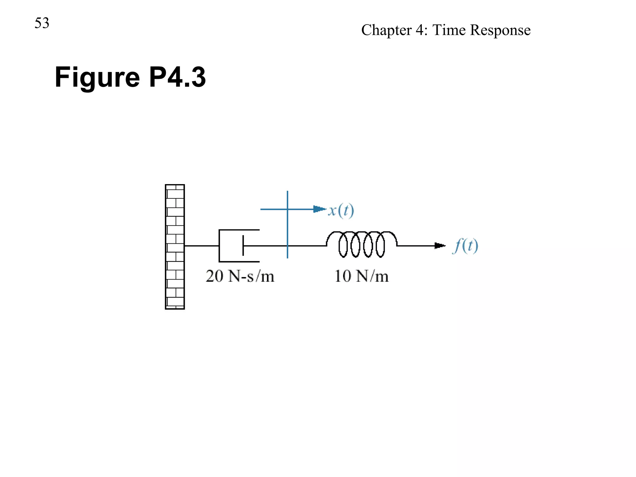
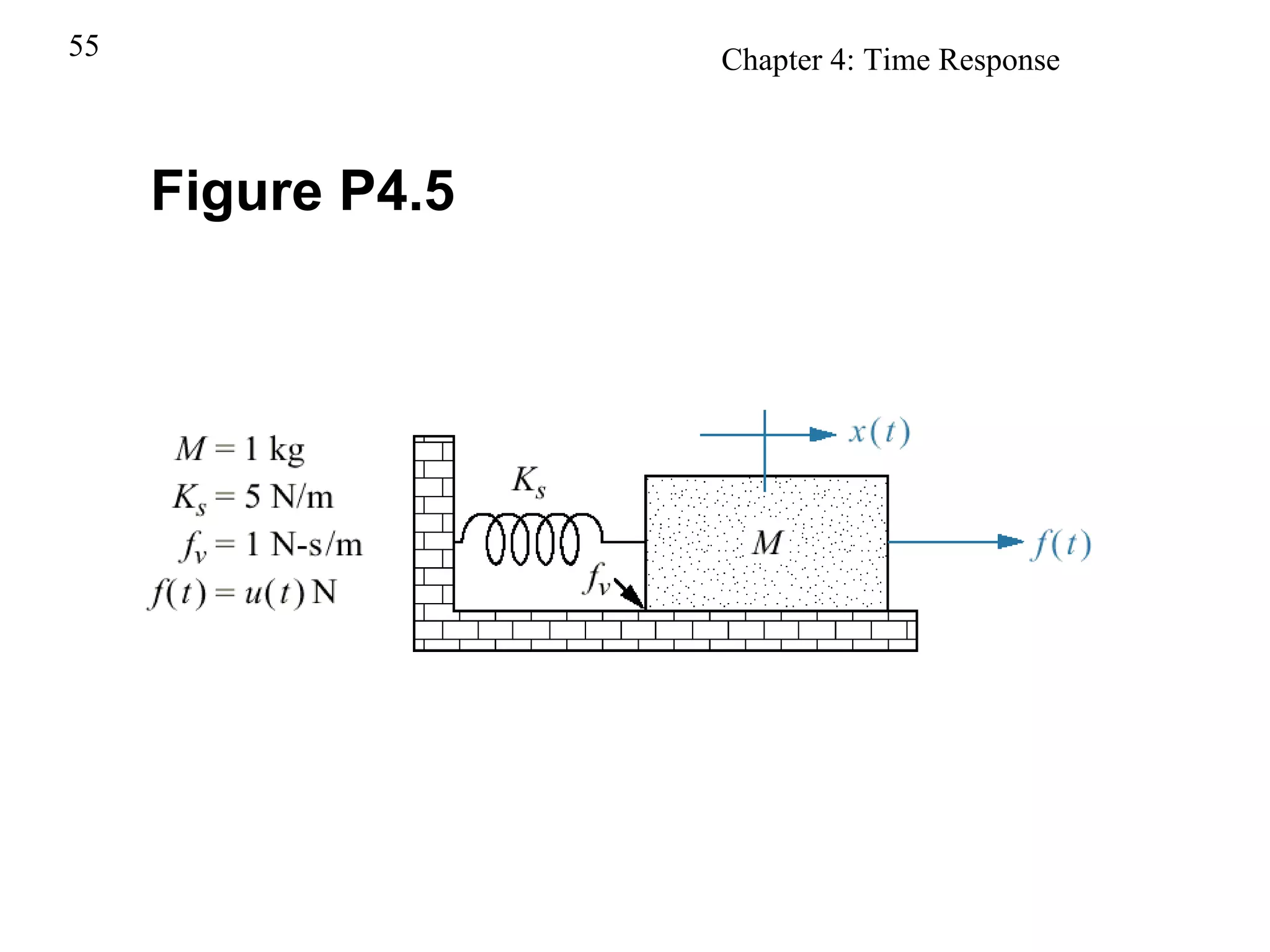
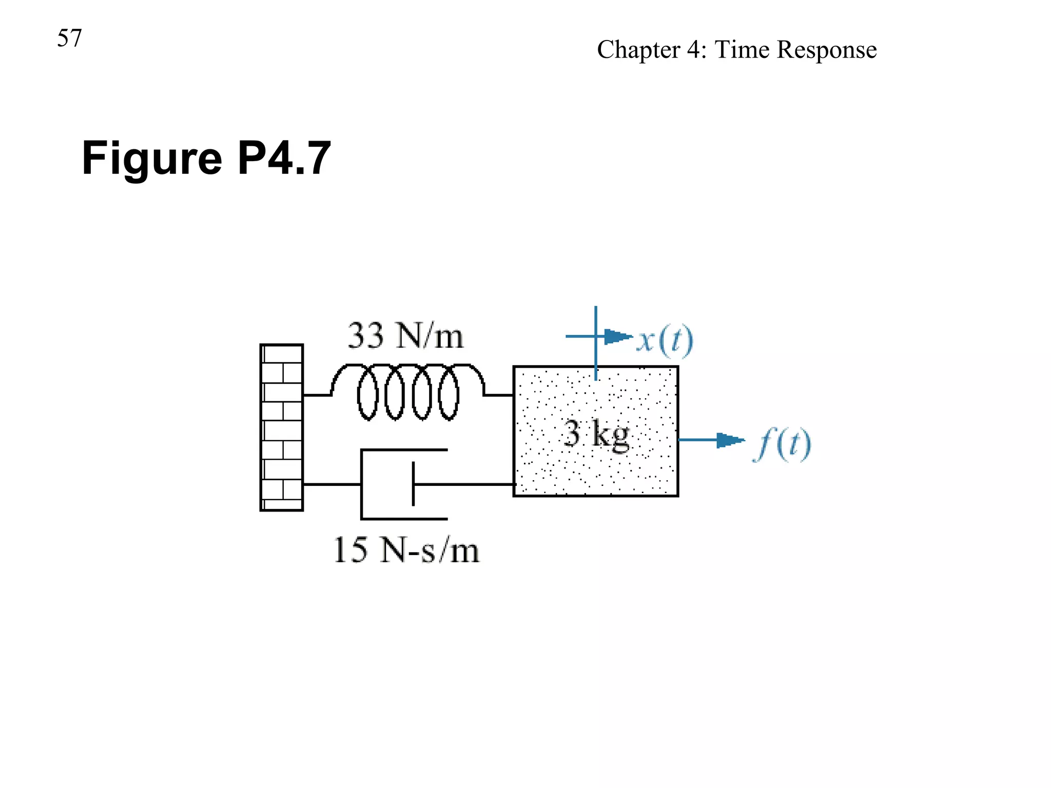
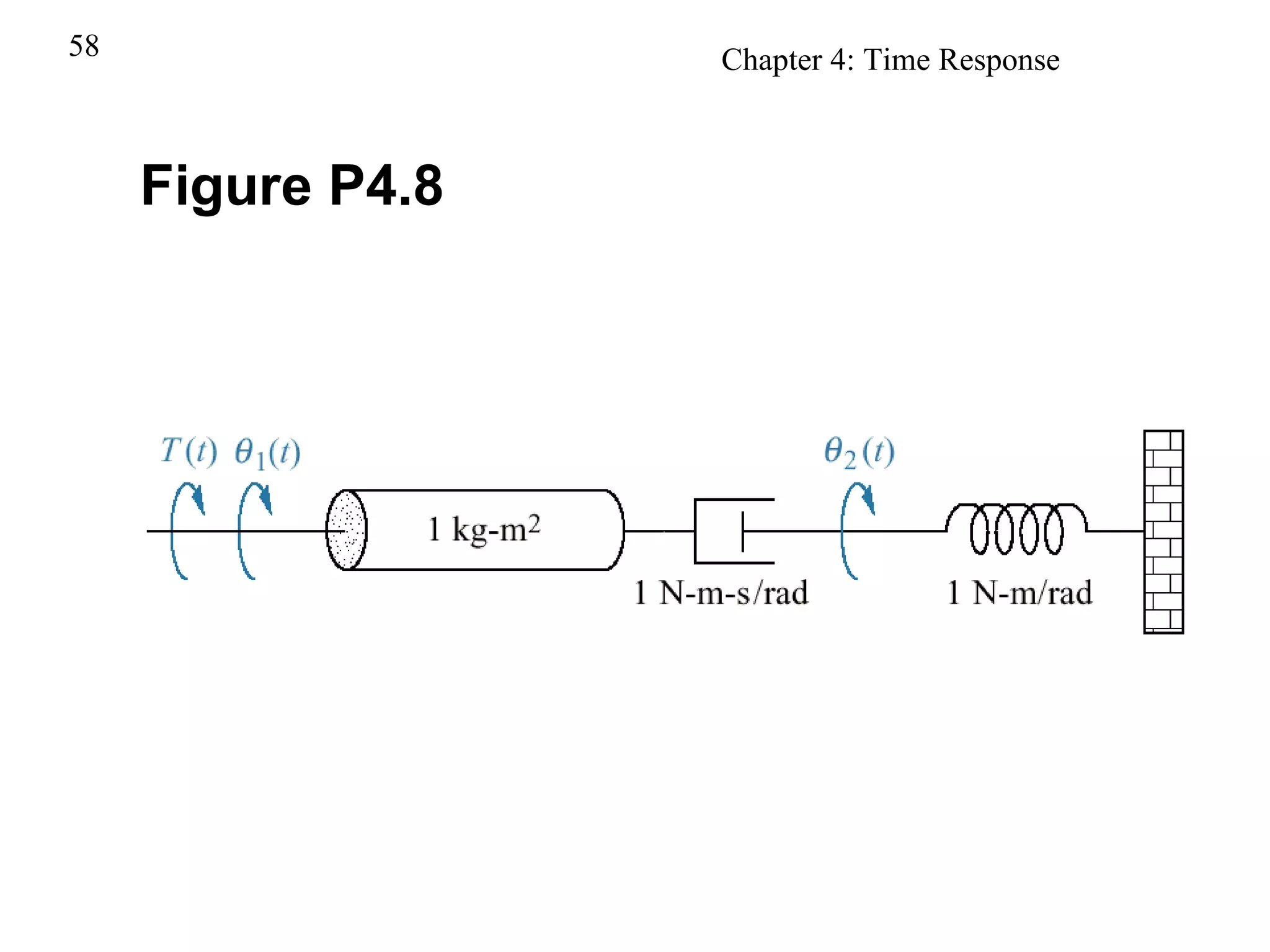
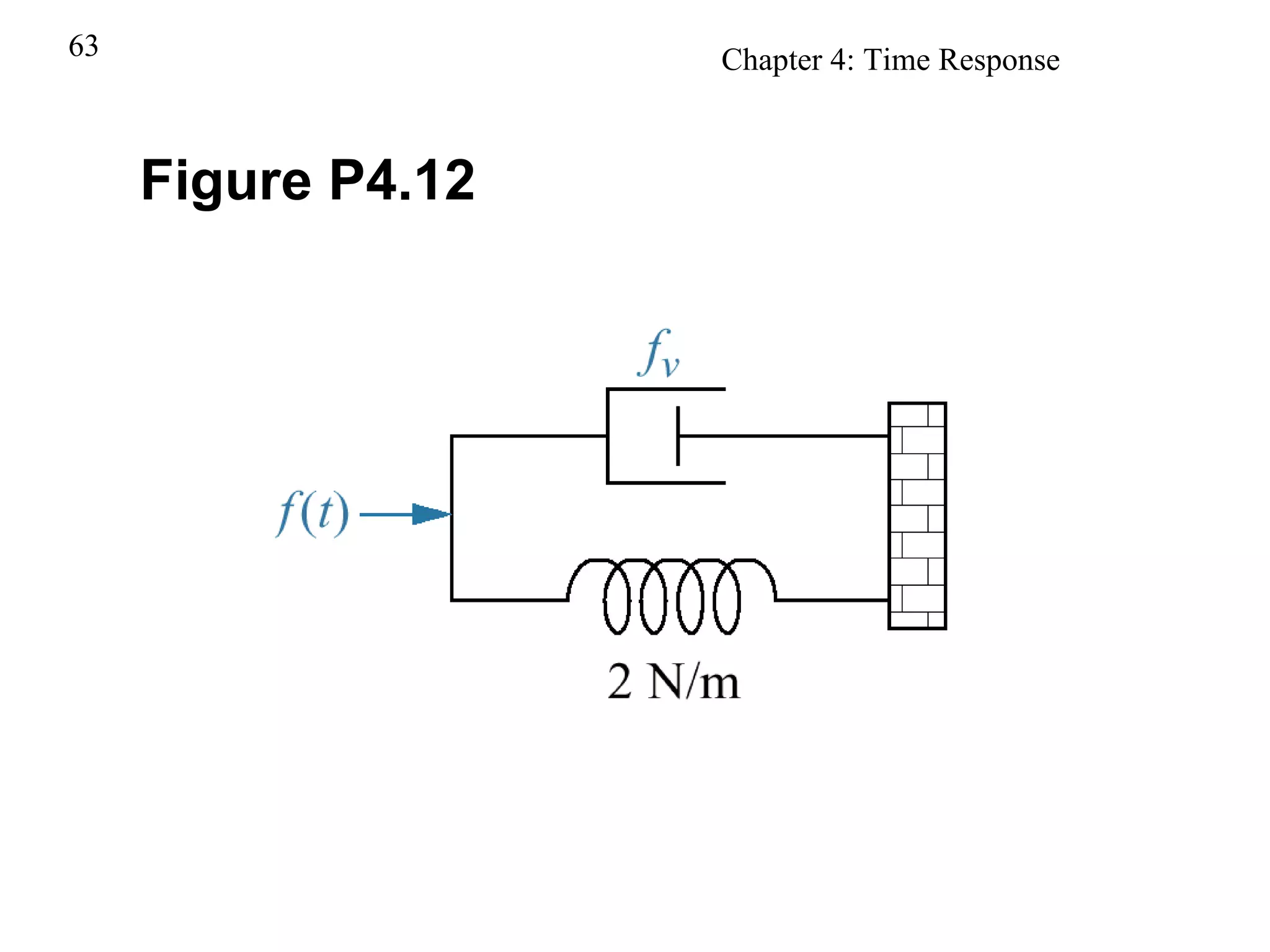
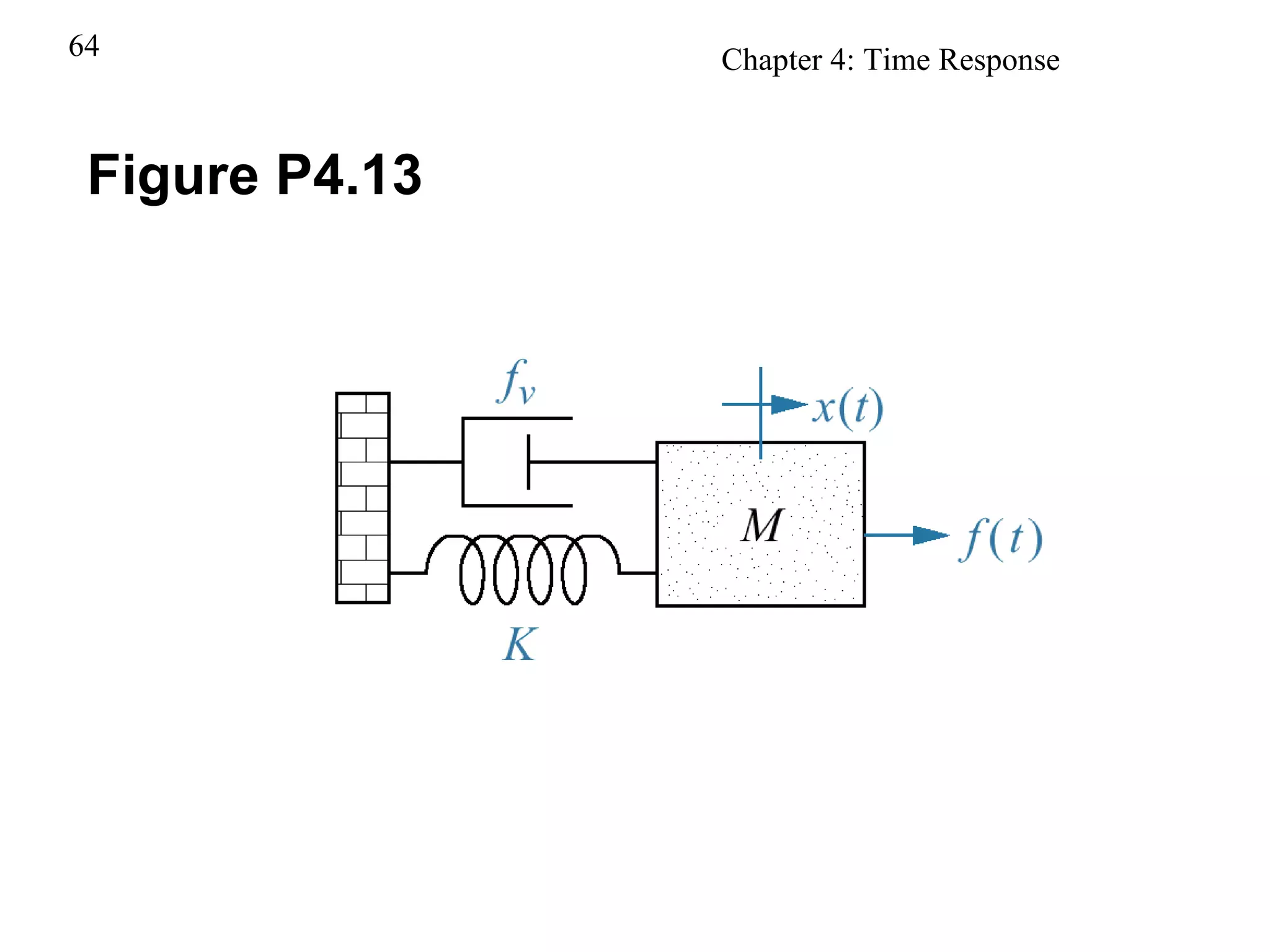
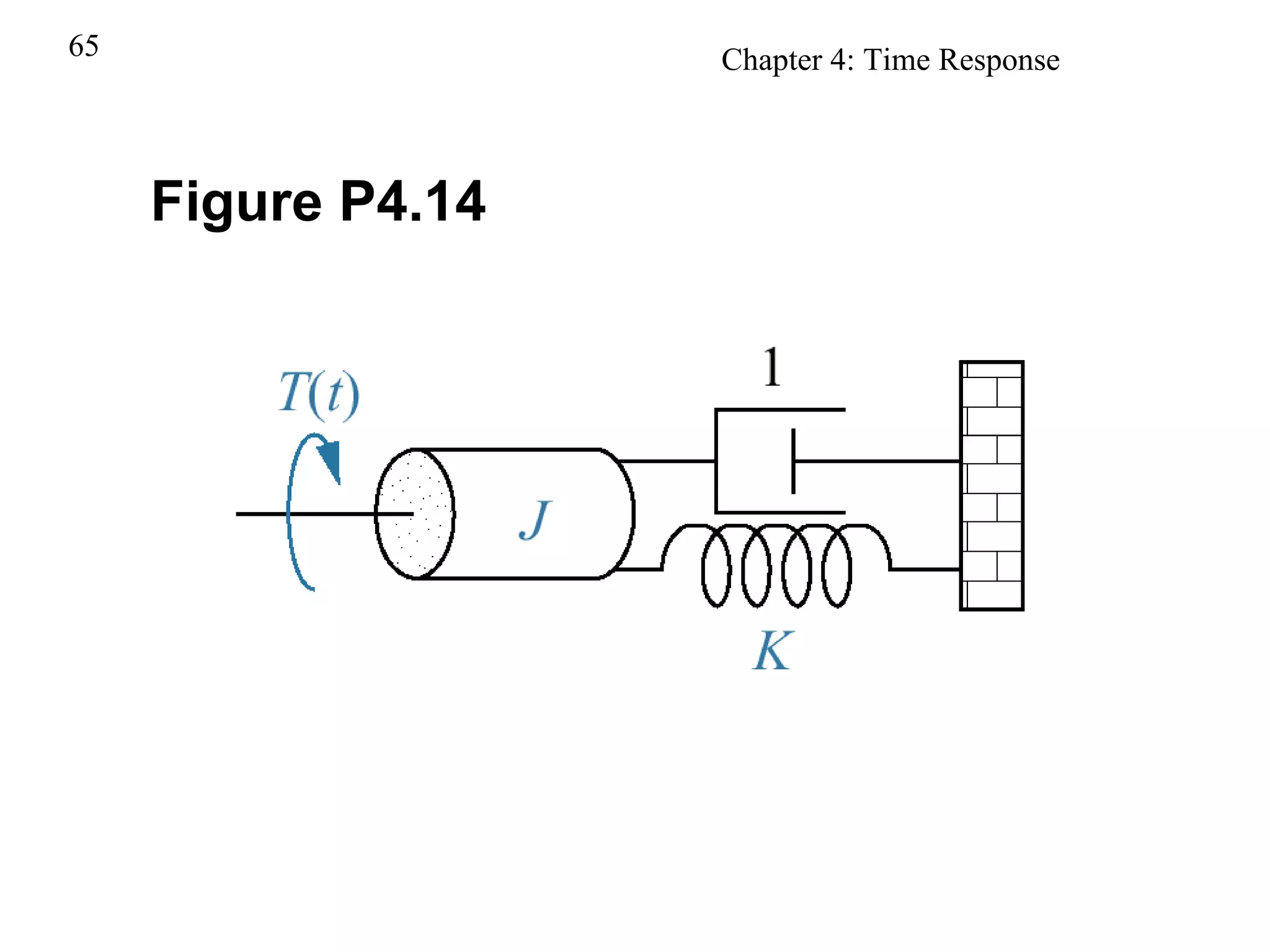
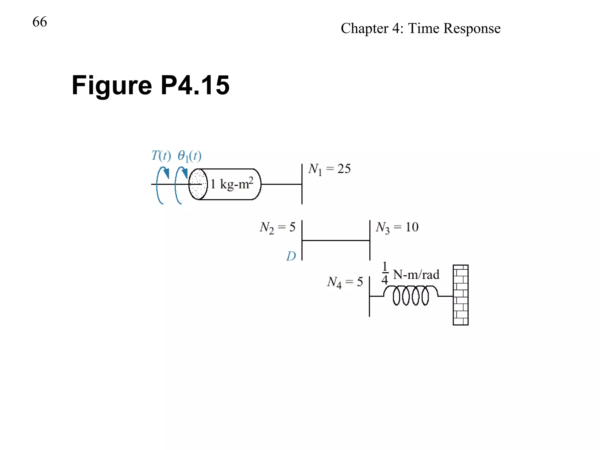
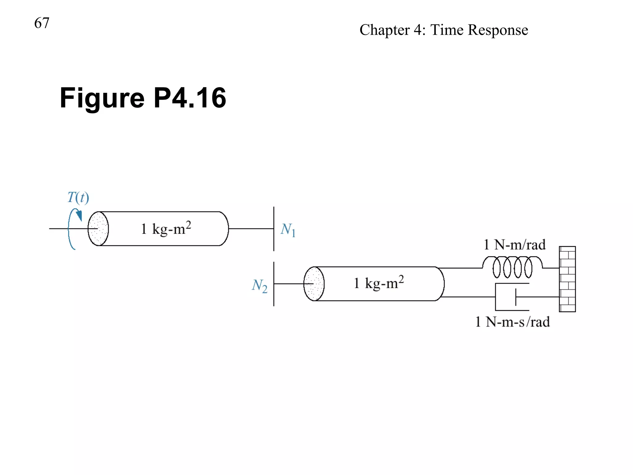
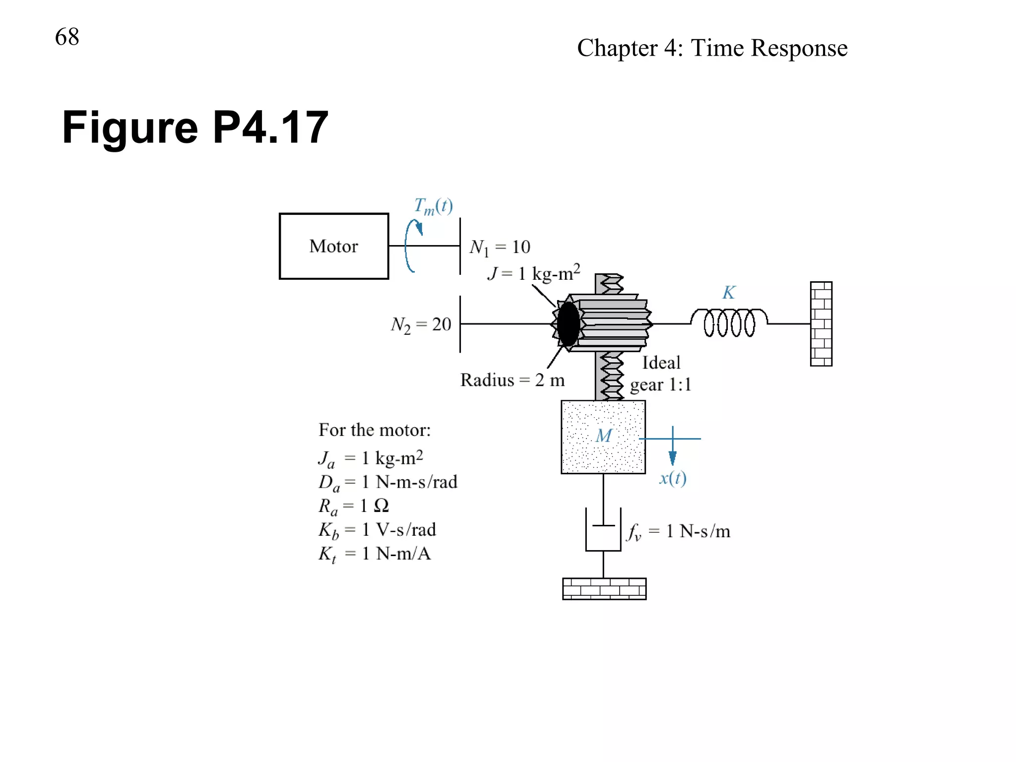
Demonstrates a mechanical system example for understanding control responses.
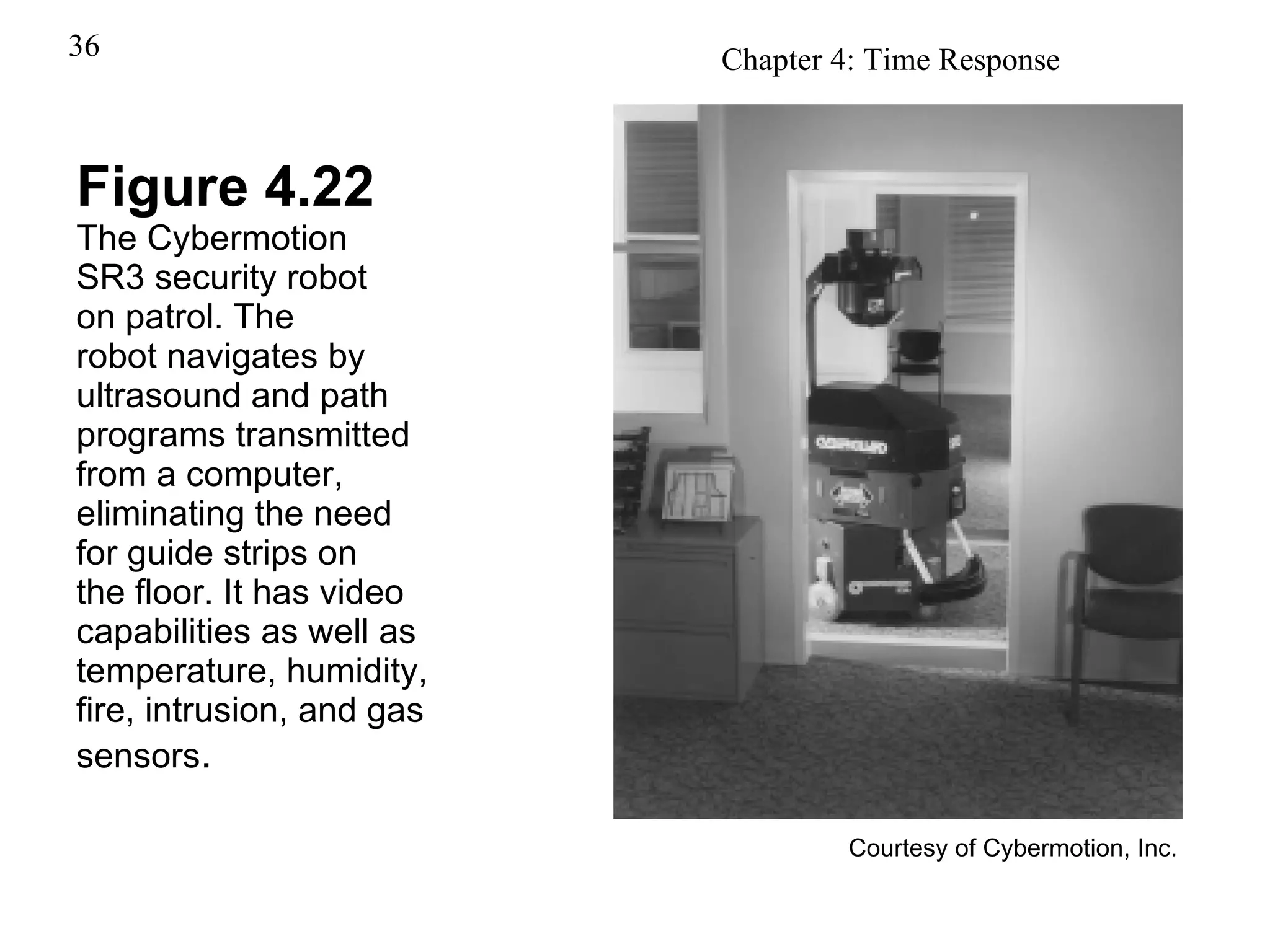
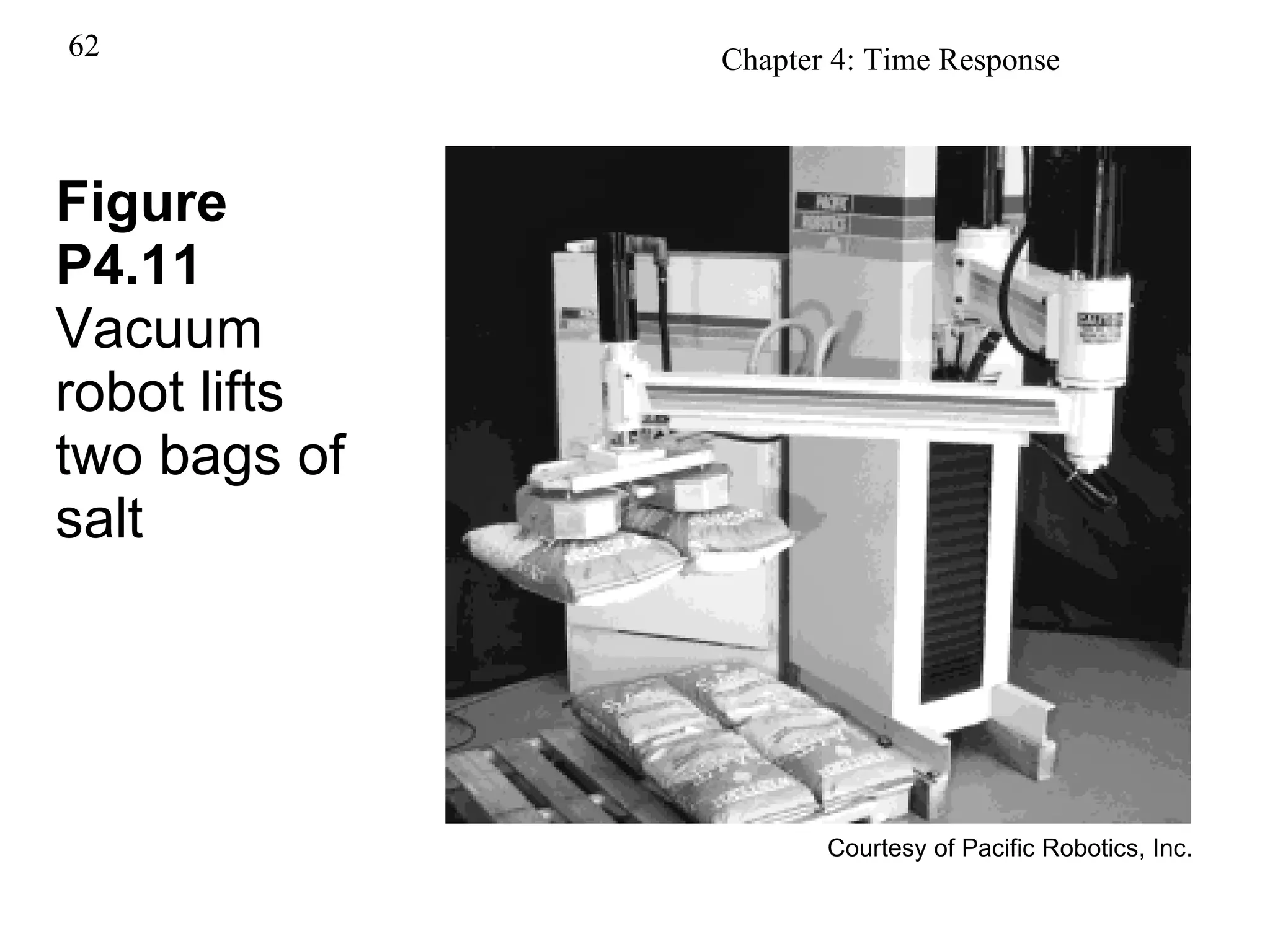
Explains the capabilities and functionalities of an advanced security robot navigating autonomously.
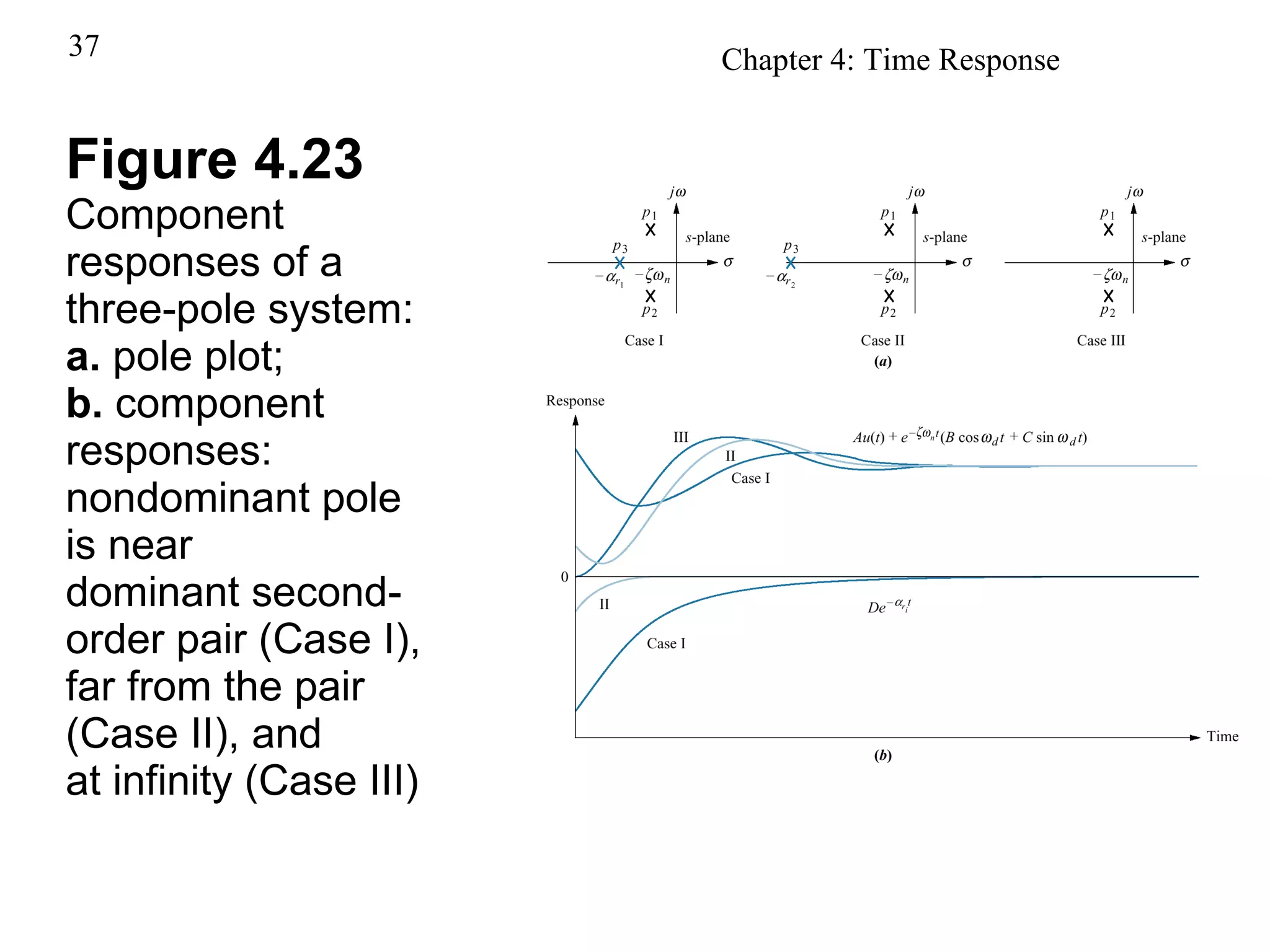
Analyzes the response characteristics of systems with three poles and various configurations.
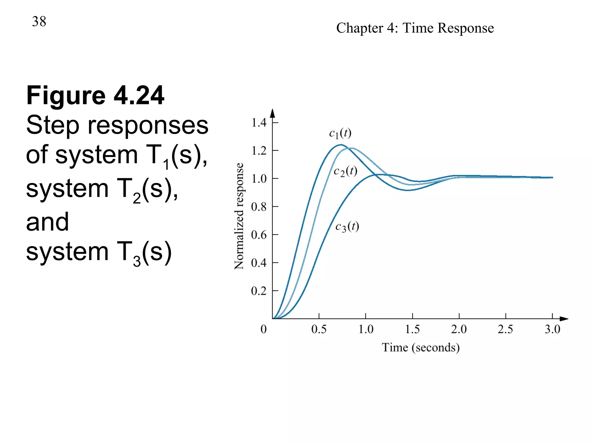
Displays step response comparisons across multiple system configurations.
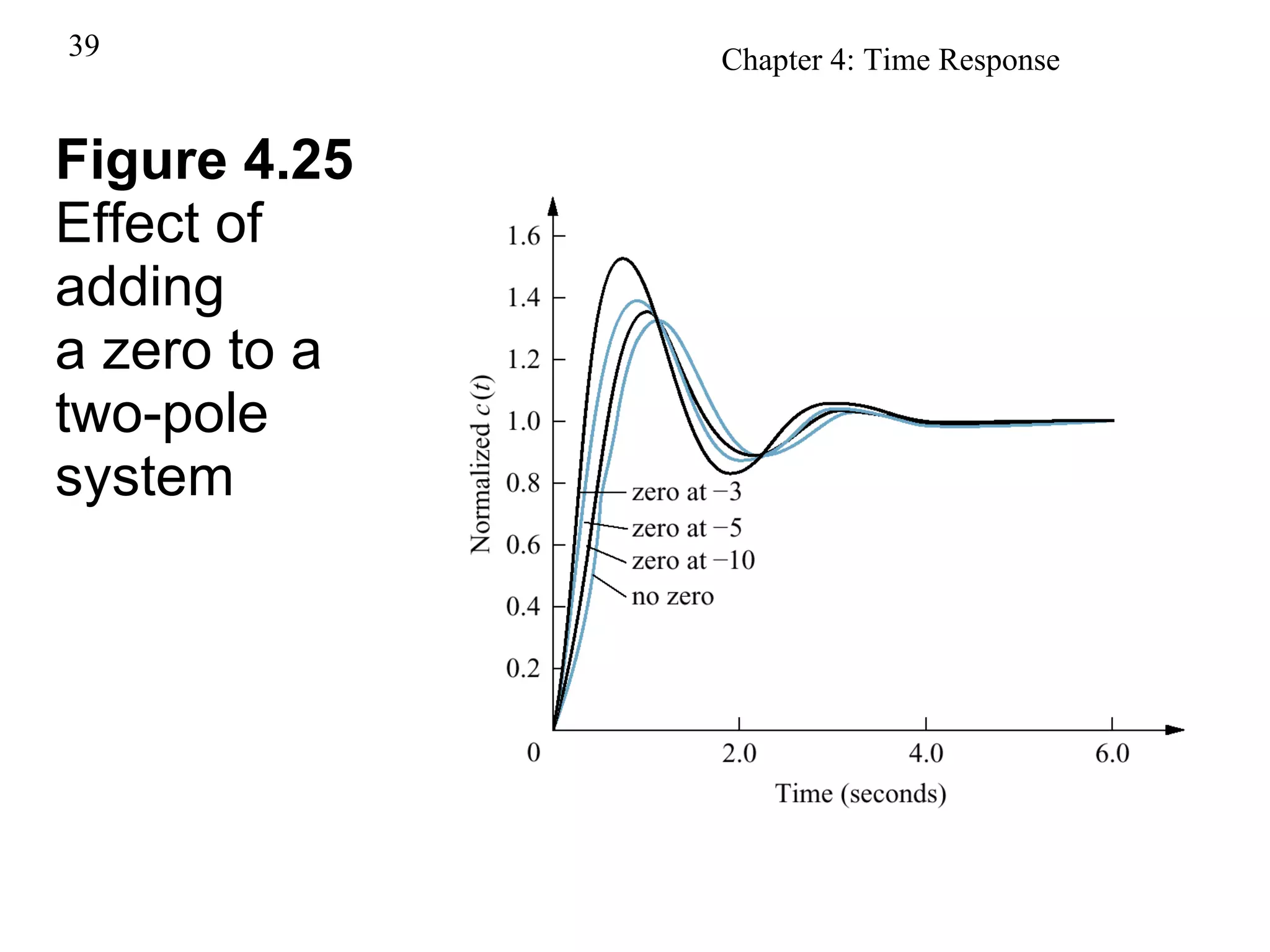
Examines how adding a zero affects the step response of a two-pole system.
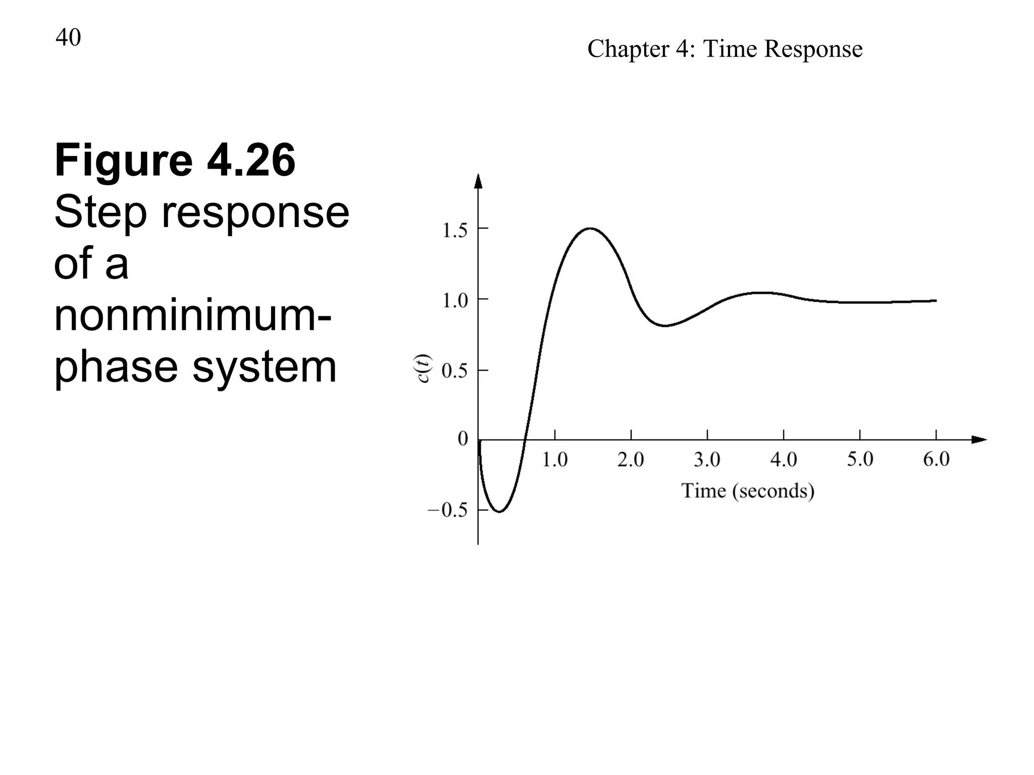
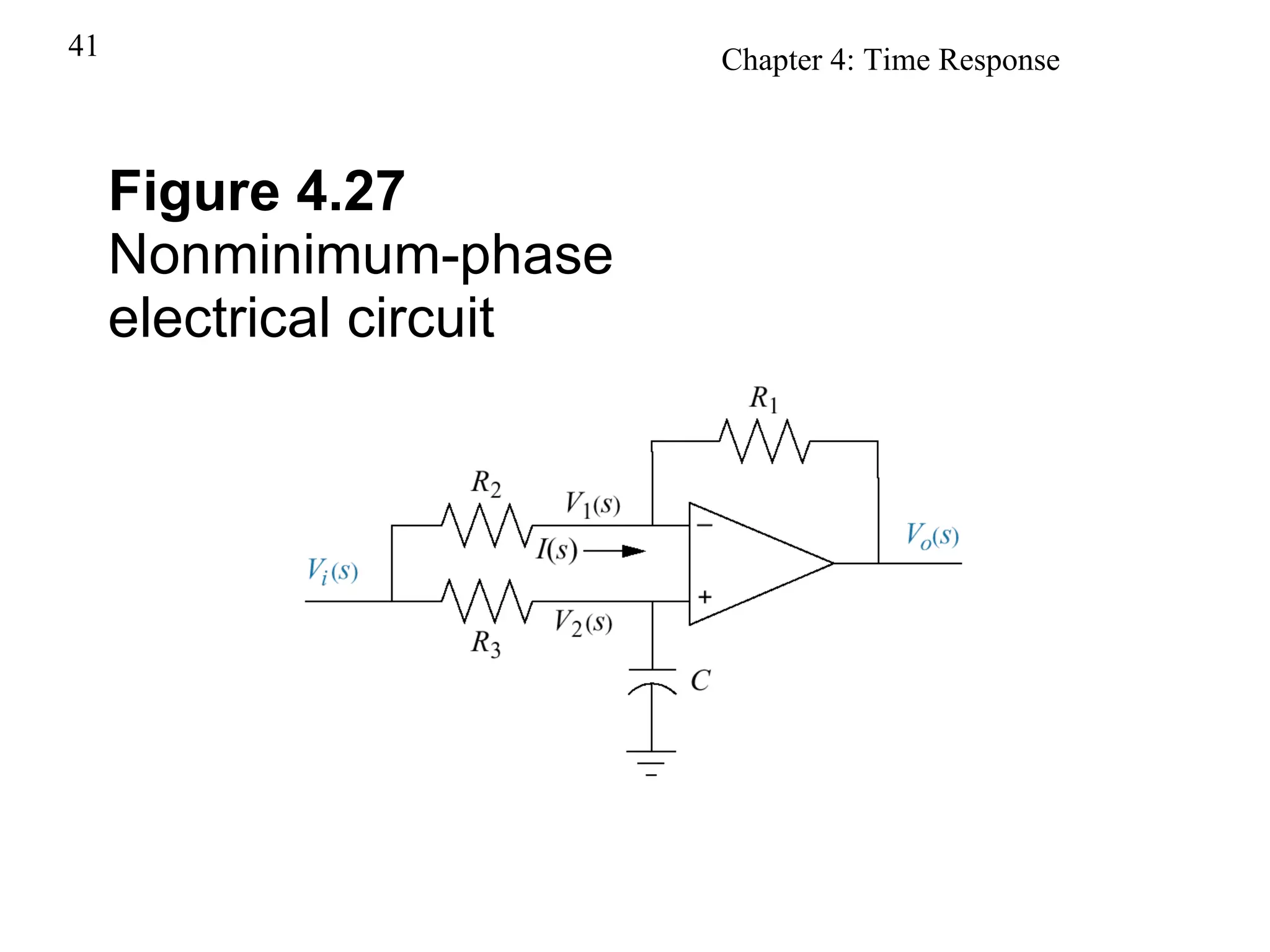
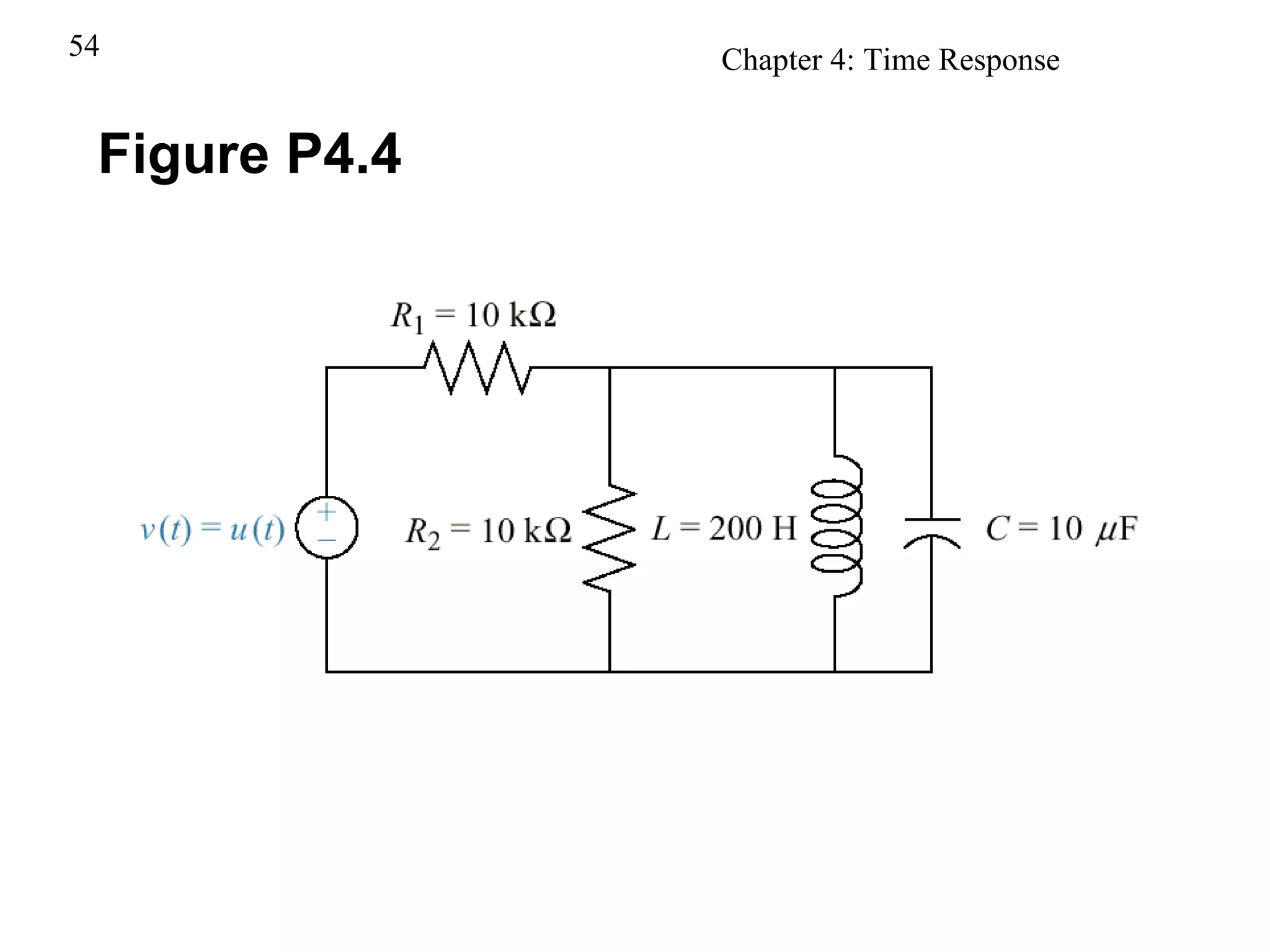
Studies the step response characteristics of a nonminimum-phase circuit.
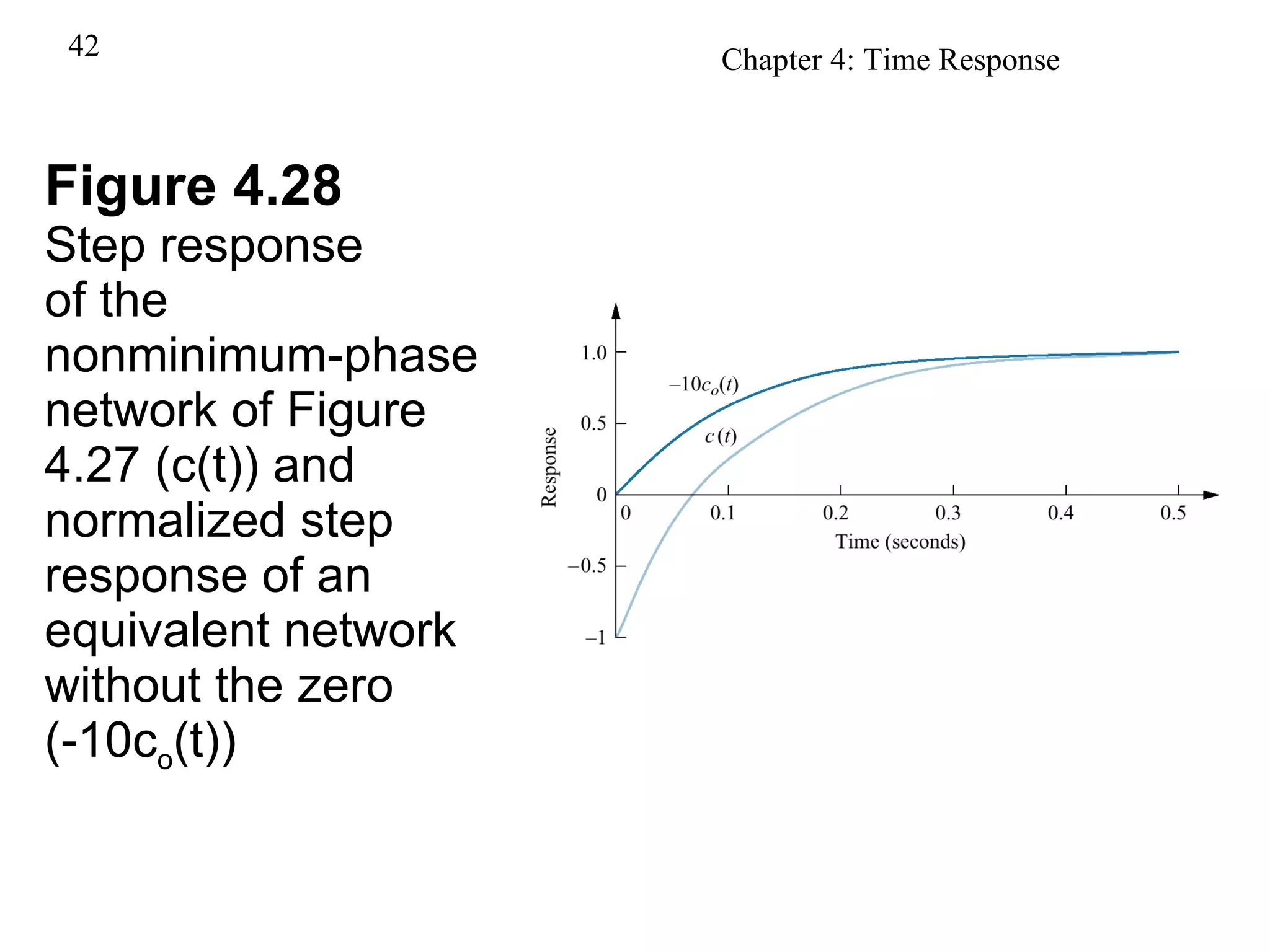
Compares step responses of nonminimum-phase networks with equivalent systems lacking zeros.
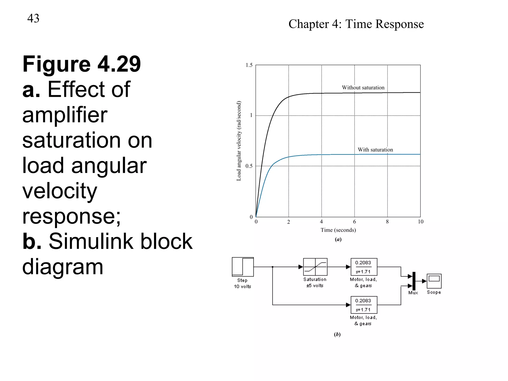
Investigates how amplifier saturation affects load angular velocity responses.
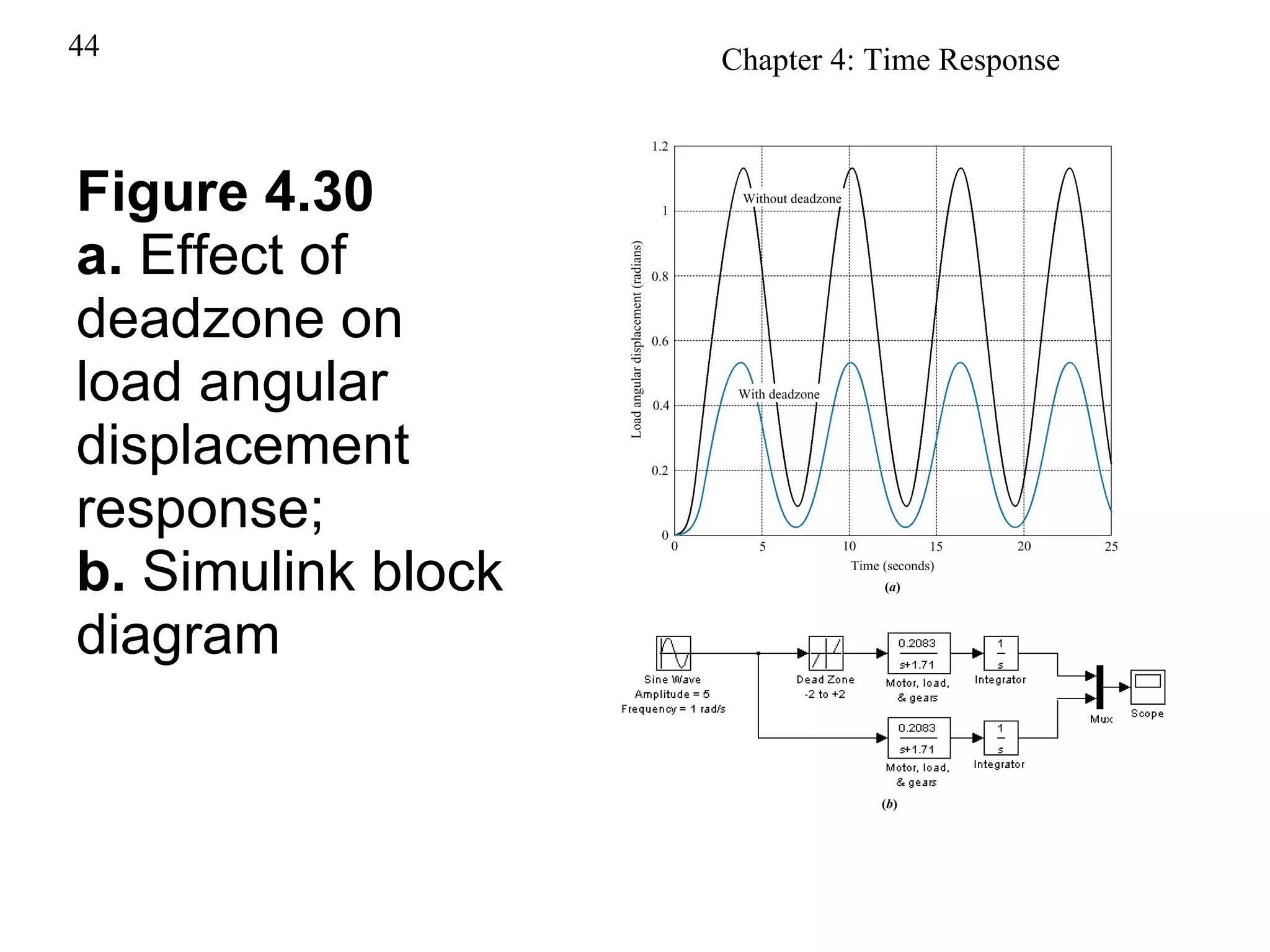
Discusses how deadzone phenomena impact load angular displacement responses.
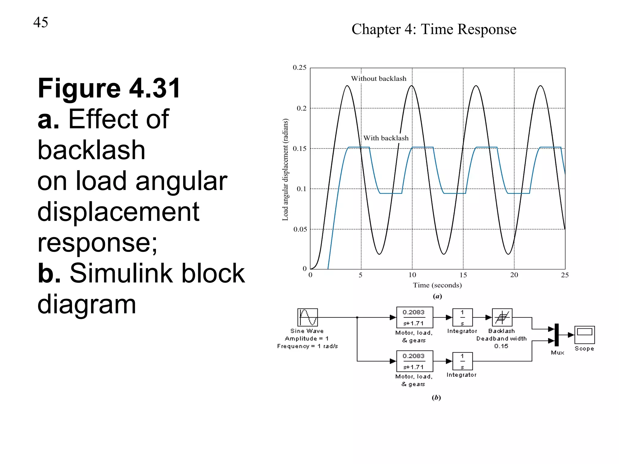
Explores how backlash affects load angular displacement and presents system diagrams.
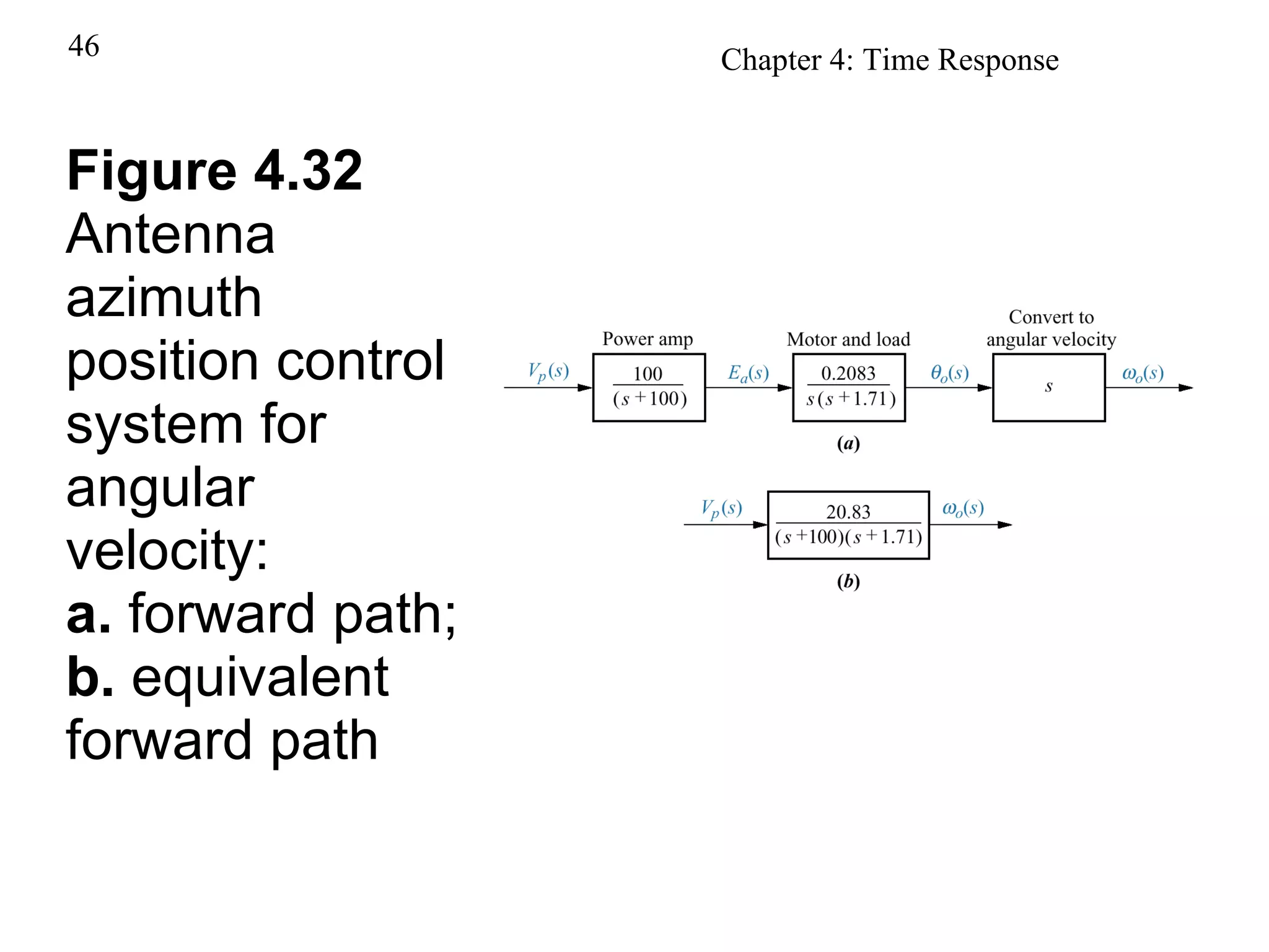
Analyzes the antenna azimuth position control system and its functional pathways.
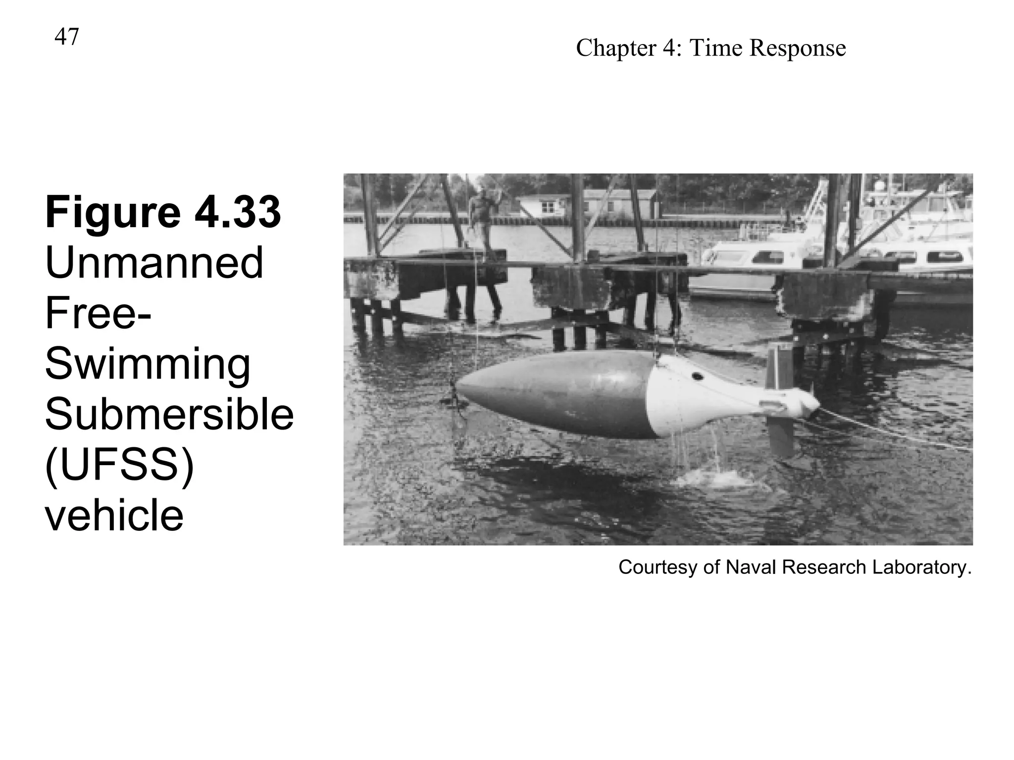
Highlights the design and capabilities of the Unmanned Free-Swimming Submersible (UFSS) vehicle.
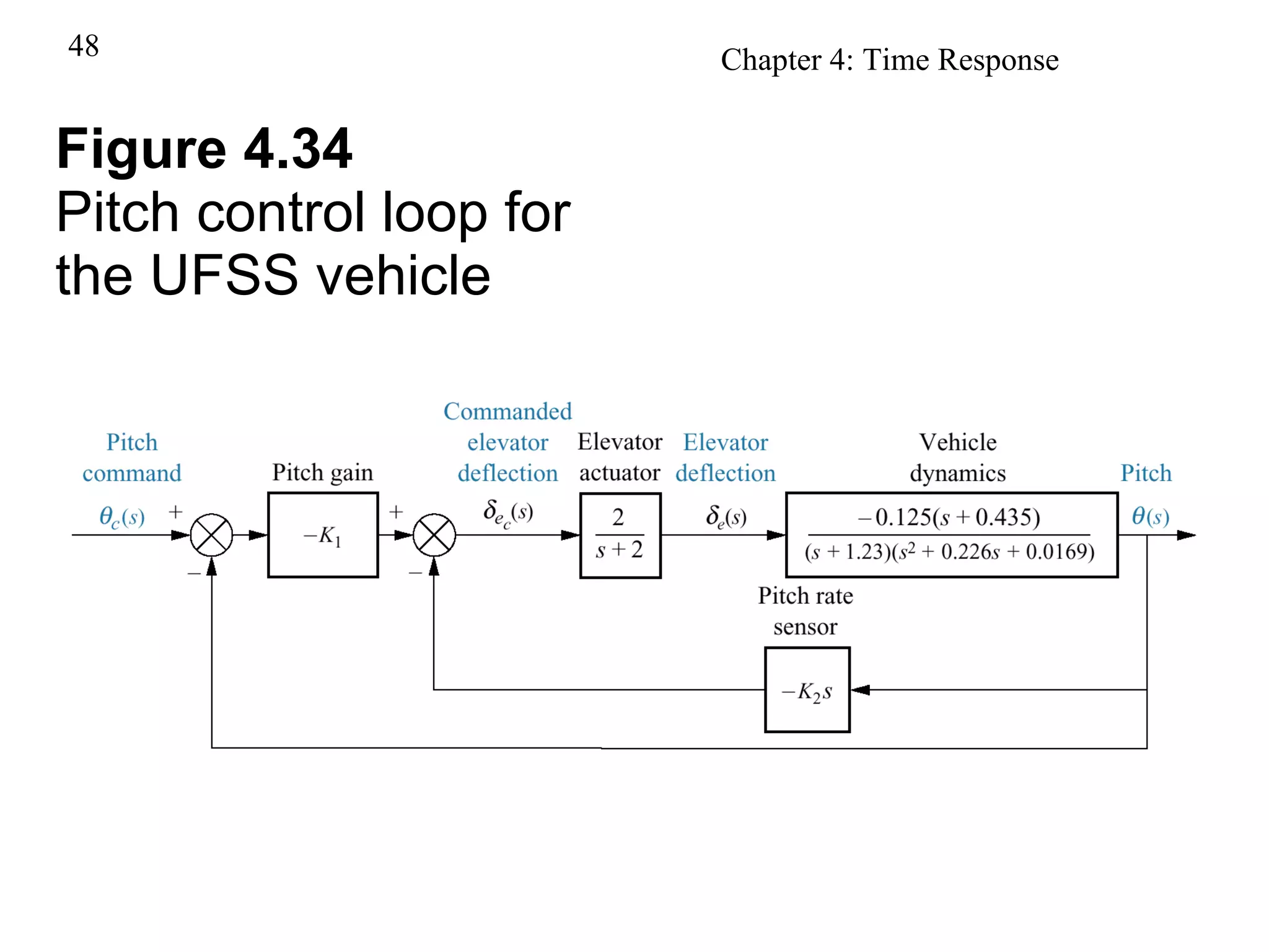
Details the pitch control loop mechanisms involved in the UFSS vehicle operations.
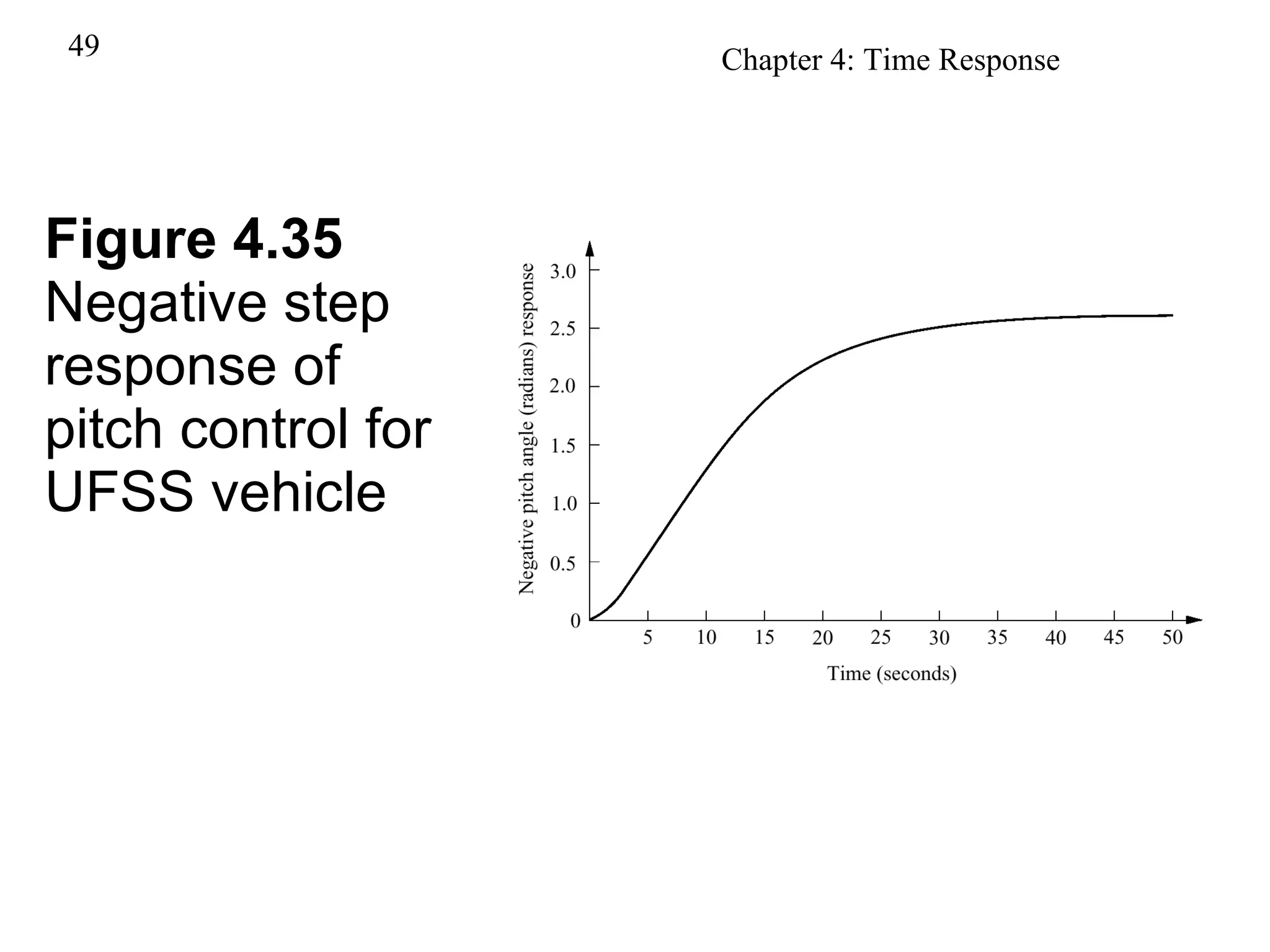
Showcases a negative step response analysis of pitch control for the UFSS vehicle.
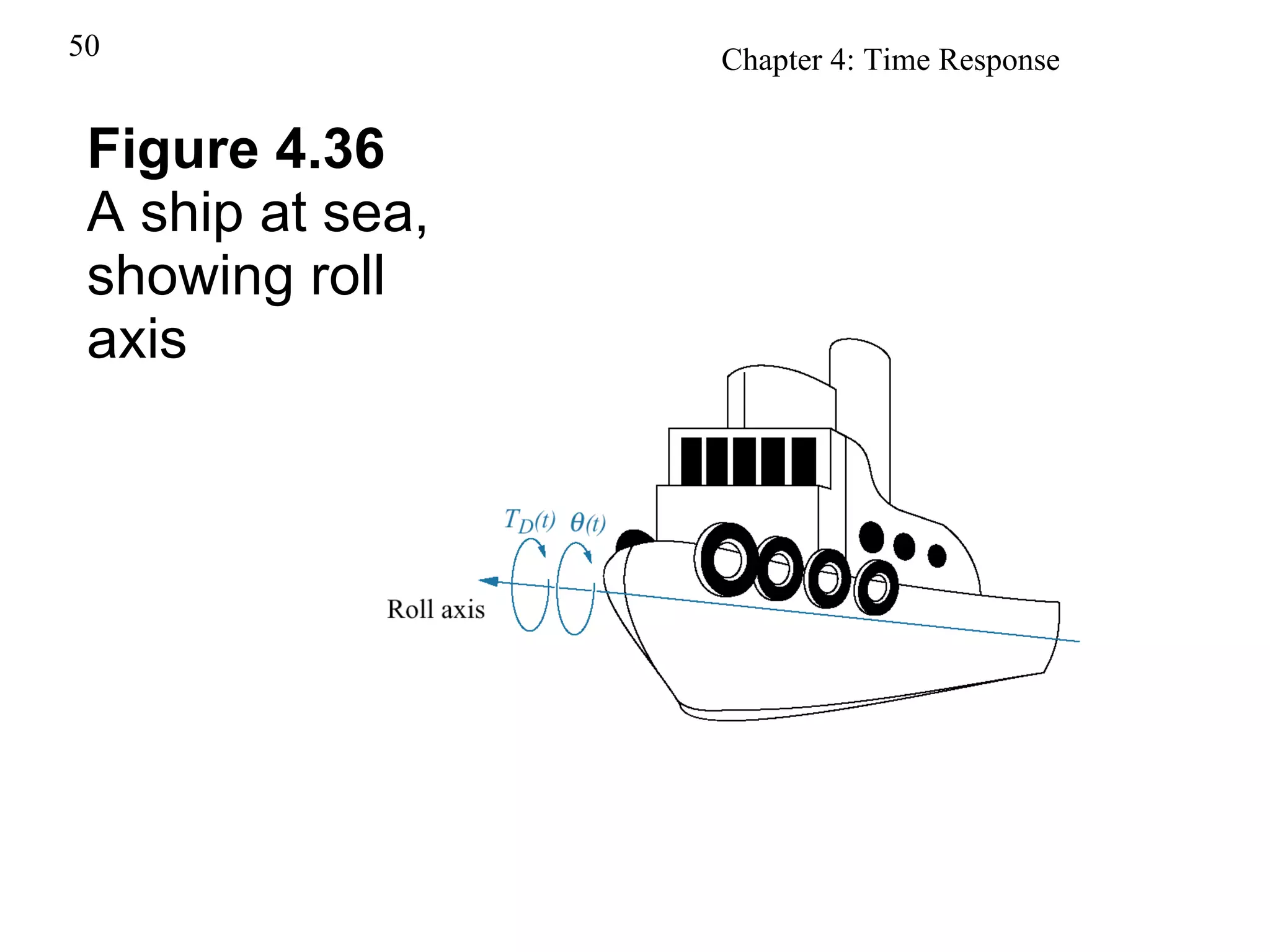
Explains systems and dynamics involved in the roll axis of ships.
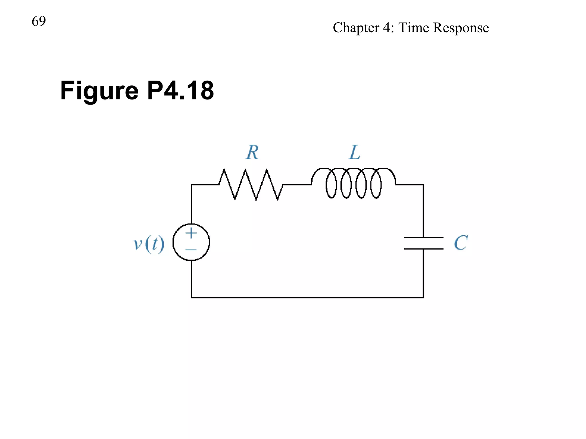
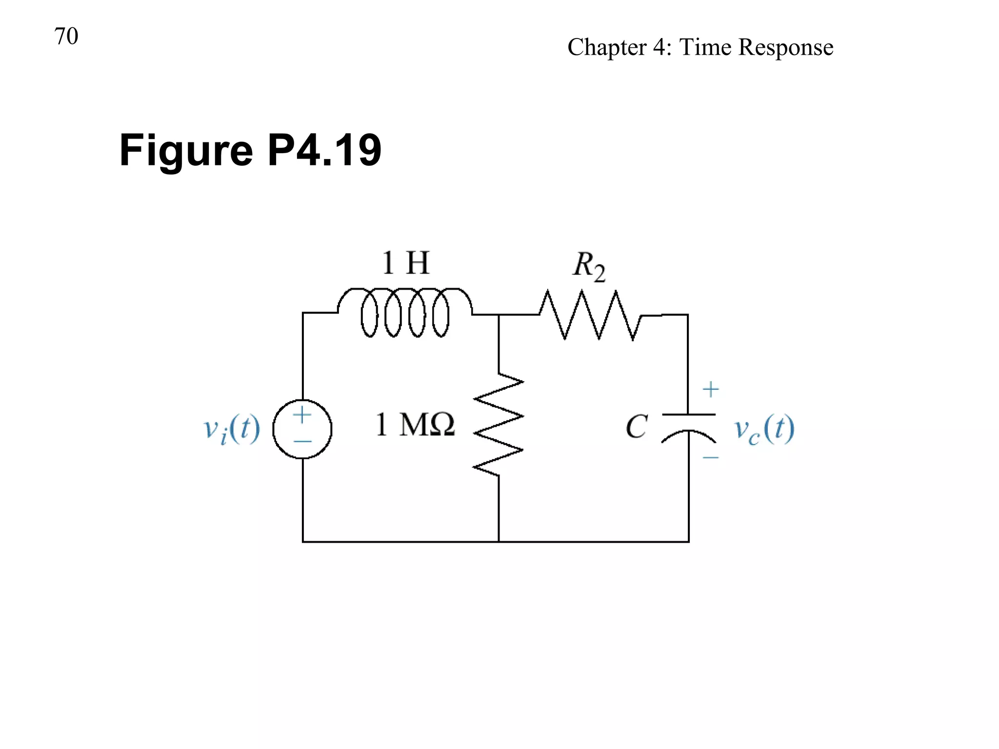
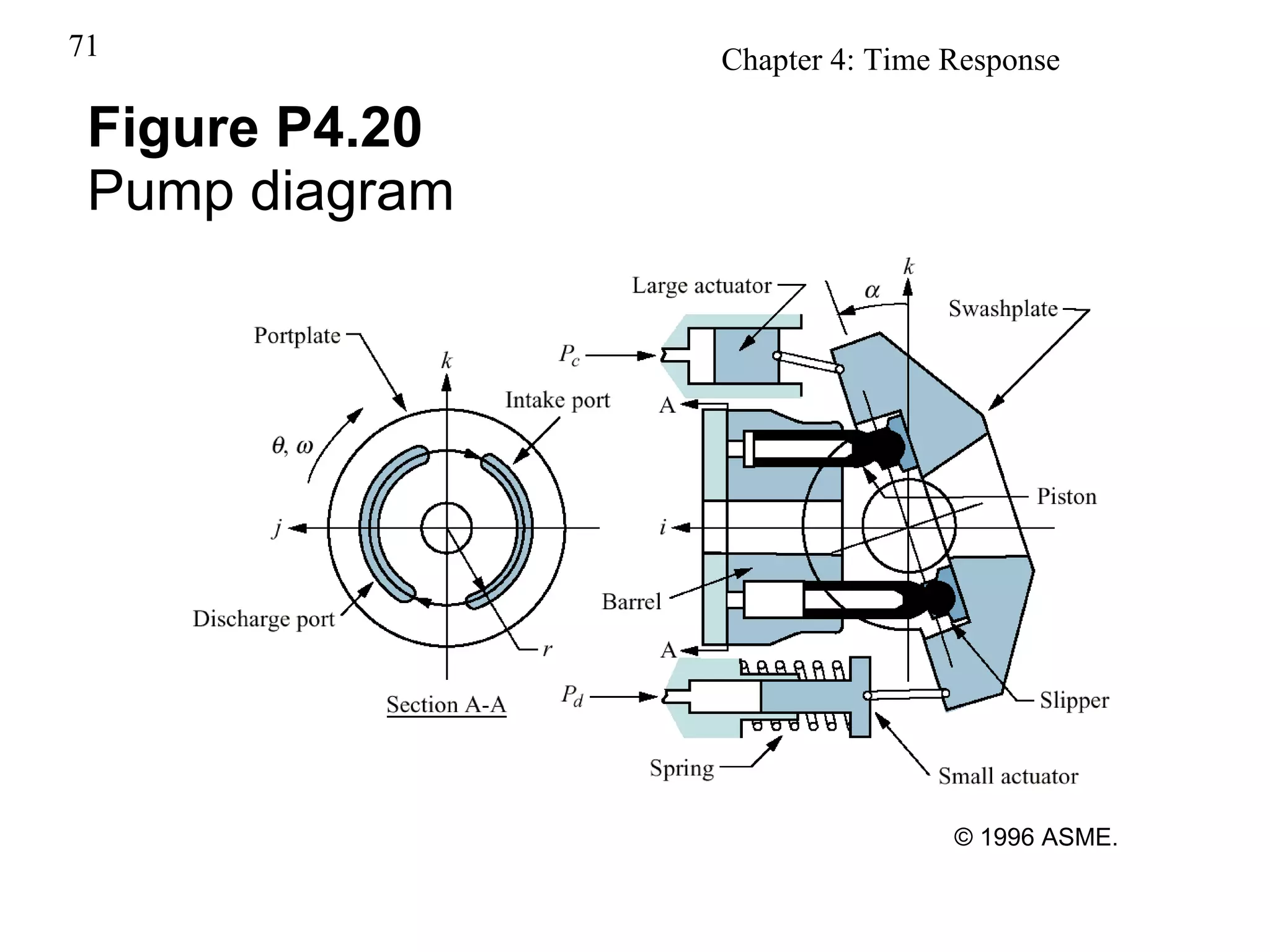
Figures and diagrams relevant to the overall analysis within the chapter context.


![Circuit Network Analysis - [Chapter5] Transfer function, frequency response, ...](https://cdn.slidesharecdn.com/ss_thumbnails/ch5-150613063859-lva1-app6891-thumbnail.jpg?width=640&height=640&fit=bounds)