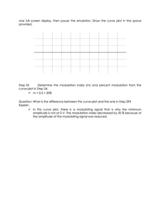
SlideShare a Scribd company logo
1 of 19
NATIONAL COLLEGE OF SCIENCE AND TECHNOLOGY
                Amafel Building, Aguinaldo Highway Dasmariñas City, Cavite


                                Experiment No. 5
                             AMPLITUDE MODULATION


Maala, Michelle Anne C.                                         August 09. 2011
Signal Spectra and Signal Processing/BSECE 41A1                 Score:


                               Engr. Grace Ramones
                                      Instructor
OBJECTIVES:
  1) Demonstrate an amplitude-modulated carrier in the time domain for different
 modulation indexes and modulating frequencies.
  2) Determine the modulation index and percent modulation of an amplitude-
 modulated carrier from the time domain curve plot.
    3) Demonstrate an amplitude-modulated carrier in the frequency domain for
 different modulation indexes and modulating frequencies.
   4) Compare the side-frequency voltage levels to the carrier voltage level in an
 amplitude-modulated carrier for different modulation indexes.
  5) Determine the signal bandwidth of an amplitude-modulated carrier for different
 modulating signal frequencies.
    6) Demonstrate how a complex modulating signal generates many side
 frequencies to form the upper and lower sidebands.
SAMPLE COMPUTATIONS:


Step 3


Step 4


Step 7


Step 8


Step 9


Step 9 Q


Step 10


Step 10 Q


Step 12


Step 13


Step 13 Q
Step 16


Step 17


Step 19


Step 20


Step 21 Q


Step 26


Step 28


Step 30


Step 35
DATA SHEET:
Materials
Two function generators
One dual-trace oscilloscope
One spectrum analyzer
One 1N4001 diode
One dc voltage supply
One 2.35 nF capacitor
One 1 mH inductor
Resistors: 100 Ω, 2 kΩ, 10 kΩ, 20 kΩ

Theory:
The primary purpose of a communications system is to transmit and receive information
such as audio, video, or binary data over a communications medium or channel. The
basic components in a communications system are the transmitter communications
medium or channel, and the receiver. Possible communications media are wire cable,
fiber optic cable, and free space. Before the information can be transmitted, it must be
converted into an electrical signal compatible with the communications medium, this is
the purpose of the transmitter while the purpose of the receiver is to receive the
transmitted signal from the channel and convert it into its original information signal
form. Is the original electrical information signal is transmitted directly over the
communications channel, it is called baseband transmission. An example of a
communications system that uses baseband transmission is the telephone system.
Noise is defined as undesirable electrical energy that enters the communications
system and interferes with the transmitted message. All communication systems are
subject to noise in both the communication channel and the receiver. Channel noise
comes from the atmosphere (lightning), outer space (radiation emitted by the sun and
stars), and electrical equipment (electric motors and fluorescent lights). Receiver noise
comes from electronic components such as resistors and transistors, which generate
noise due to thermal agitation of the atoms during electrical current flow. In some cases
obliterates the message and in other cases it results in only partial interference.
Although noise cannot be completely eliminated, it can be reduced considerably.
Often the original electrical information (baseband) signal is not compatible with the
communications medium. In that case, this baseband signal is used to modulate a
higher-frequency sine wave signal that is in a frequency spectrum that is compatible
with the communications medium. This higher-frequency sine wave signal is called a
carrier. When the carrier frequency is in the electromagnetic spectrum it is called a
radio frequency (RF) wave, and it radiates into space more efficiently and propagates
a longer distance than a baseband signal. When information is transmitted over a fiber
optic cable, the carrier frequency is in the optical spectrum. The process of using a
baseband signal to modulate a carrier is called broadband transmission.
There are basically three ways to make a baseband signal modulate a sine wave
carrier: amplitude modulation (AM), frequency modulation (FM), and phase
modulation (PM). In amplitude modulation (AM), the baseband information signal
varies the amplitude of the higher-frequency carrier. In frequency modulation (FM), the
baseband information signal varies the frequency of the higher-frequency carrier and
the carrier amplitude remains constant. In phase modulation (PM), the baseband
information signal varies the phase of the high-frequency carrier. Phase modulation
(PM) is different fork of frequency modulation and the carrier is similar in appearance to
a frequency-modulated signal carrier. Therefore, both FM and PM are often referred to
as an angle modulation. In this experiment, you will examine the characteristics of
amplitude modulation (AM).
In amplitude modulation, the carrier frequency remains constant, but the instantaneous
value of the carrier amplitude varies in accordance with the amplitude variations of the
modulating signal. An imaginary line joining the peaks of the modulated carrier
waveform, called the envelope, is the same shape as the modulating signal with the
zero reference line coinciding with the peak value of the unmodulated carrier. The
relationship between the peak voltage of the modulating signal (Vm) and the peak
voltage of the unmodulated carrier (Vc) is the modulation index (m), therefore,


Multiplying the modulation index (m) by 100 gives the percent modulation. When the
peak voltage of the modulating signal is equal to the peak voltage of the
unmodulated carrier, the percent modulation is 100%. An unmodulated carrier has a
percent modulation of 0%. When the peak voltage of the modulating signal (Vm)
exceeds the peak voltage of the unmodulated carrier (Vc) overmodulation will occur,
resulting in distortion of the modulating (baseband) signal when it is recovered from the
modulated carrier. Therefore, if it is important that the peak voltage of the modulating
signal be equal to or less than the peak voltage of the unmodulated signal carrier
(equal to or less than 100% modulation) with amplitude modulation.
Often the percent modulation must be measured from the modulated carrier displayed
on an oscilloscope. When the AM signal is displayed on an oscilloscope, the modulation
index can be computed from


where Vmax is the maximum peak-to-peak voltage of the modulated carrier and Vmin is
the minimum peak-to-peak voltage of the modulated carrier. Notice that when Vmax =
0, the modulation index (m) is equal to 1 (100% modulation), and when Vmin = Vmax, the
modulation index is equal to 0 (0% modulation).
when a single-frequency sine wave amplitude modulates a carrier, the modulating
process causes two side frequencies to be generated above and below the carrier
frequency be an amount equal to the modulating frequency (fm). The upper side
frequency (fuse) and the lower side frequency (fluff) can be determine from


A complex modulating signal, such as a square wave, consists of a fundamental sine
wave frequency and many harmonics, causing many side frequencies to be
generated. The highest upper side frequency and the lowest lower side frequency are
determined be the highest harmonic frequency (fm (max), and the highest lower side
frequency and the lower upper side frequency are determined by the lowest harmonic
frequency (fm (min)). The band of frequencies between (fC + fm (min)) and (fC + fm (max)) is
called the upper sideband. The band of frequencies between (fC – fm (min)) and (fC – fm
(max)) is called the lowers sideband. The difference between the highest upper side
frequency (fC + fm (max)) and the lowest lower side frequency (fC – fm (max)) is called the
bandwidth occupied by the modulated carrier. Therefore, the bandwidth (BW) can be
calculated from


This bandwidth occupied by the modulated carrier is the reason a modulated carrier is
referred to as broadband transmission.
The higher the modulating signal frequencies (meaning more information is being
transmitted) the wider the modulated carrier bandwidth. This is the reason a video
signal occupies more bandwidth than an audio signal. Because signals transmitted on
the same frequency interfere with one another, this carrier bandwidth places a limit on
the number of modulated carriers that can occupy a given communications channel.
Also, when a carrier is overmodulated, the resulting distorted waveshape generates a
harmonic that generate additional side frequencies. This causes the transmitted
bandwidth to increase and interfere with other signals. This harmonic-generated
sideband interference is called splatter.
When an AM signal on an oscilloscope, it is observed in the time domain (voltage as a
function time). The time domain display gives no indication of sidebands. In order to
observe the sidebands generated by the modulated carrier, the frequency spectrum of
the modulated carrier must be displayed in the frequency domain (sine wave voltage
levels as a function of frequency) on a spectrum analyzer.
A sine wave modulated AM signal is a composite of a carrier and two side frequencies,
and each of these signals transmits power. The total power transmitted (PT) is the sum of
each carrier power ((PC) and the power in the two side frequencies (PUSF and PUSB).
Therefore,


The total power transmitted (PT) can also be determined from the modulation index (m)
using the equation


Therefore, the total power in the side frequencies (PSF) is


and the power in each side frequency is


Notice that the power in the side frequencies depends on the modulation index
(percent modulation) and the carrier power does not depend on the modulation
index. When the percent modulation is 100% (m = 1), the total side-frequency power
(PSF) is one-half of the carrier power (PC) and the power in each side frequency (PUSF
and PLSF) is one-quarter of the carrier power (PC). When the percent modulation is 0%,
the total side-frequency power (PSF) is zero because there are no side frequencies in an
unmodulated carrier. Based on these results, it is easy to calculate that an amplitude-
modulated carrier has all of the transmitted information in the sidebands and no
information in the carrier. For 100% modulation, one-third of the total power transmitted
is in the sidebands and two-thirds of the total power is wasted in the carrier, which
contains no information. When a carrier is modulated by a complex waveform, the
combined modulation index of the fundamental and all of the harmonics determines
the power in the sidebands. In a later experiment, you will see how we can remove and
transmit the same amount of information with less power.
Because power is proportional to voltage squared, the voltage level of the frequencies
is equal to the square root of the side-frequency power. Therefore the side-frequency
voltage can be calculated from


This means that the voltage of each side frequency is equal to one-half the carrier
voltage for 100% modulation of a sine-wave modulated carrier. When a carrier is
modulated by a complex waveform, the voltage of each side frequency can
calculated from the separate modulation indexes of the fundamental and each
harmonic.
A circuit that mathematically multiplies a carrier and modulating (baseband) signal,
and then adds the carrier to the result, will produce an amplitude-modulated carrier.
Therefore, the circuit in Figure 6-1 will be used to demonstrate amplitude modulation.
An oscilloscope has been attached to the output to display the modulated carrier in
the time domain. A spectrum analyzer has been attached to the output to display the
frequency spectrum of the amplitude-modulated carrier in the frequency domain.
XSA1                          XSC1
       Modulating Signal
          XFG1
                                                                                                    Ext T rig
                                                                                                            +
                                                                                                           _
                                                                 IN T           A           B
                                                                            +       _   +       _               0
              0                MULTIPLIER       SUMMER
                   3
                                Y
                                                      C
                                X           2     A                     1
                                                            1 V/V
                           4    1 V/V 0 V             B     0V


                            Carrier
                             1 Vpk
                             100kHz
                           0 0°


Procedure
Step 1 Open circuit file Fig 6-1. This circuit will demonstrate how mathematical
       multiplication of a carrier and a modulating (baseband) signal, and then adding
       the carrier to the multiplication result, will produce an amplitude modulated
       carrier. Bring down the function generator enlargement and make sure that the
       following settings are selected: Sine Wave, Freq=5kHz, Ampl = 1V, Offset=0. Bring
       down the oscilloscope enlargement and make sure that the following settings
       are selected: Time base (Scale = 50 µs/Div, Xpos= 0, Y/T) Ch A (Scale = 1 V/Div,
       Ypos = 0, DC) Trigger (Pos edge, Level = 0, Auto).
Step 2 Run the simulation to one full screen display, then pause the simulation. Notice
       that you have displayed an amplitude-modulated carrier curve plot on the
       oscilloscope screen. Draw the curve plot in the space provided and show the
       envelope on the drawing.
Step 3 Based on the function generator amplitude (modulating sine wave voltage, Vm)
        and the voltage of the carrier sine wave (Vc), calculate the expected
        modulation index (m) and percent modulation.
         m=1 or 100%
Step 4 Determine the modulation index (m) and percent modulation from the curve
plot in Step 2.
         m=1 or 100%
Question: How did the value of the modulation index and percent modulation
determined from the curve plot compare with the expected value calculated in Step
3?
         There is no difference between the values. They have same values.
Step 5          Bring down the spectrum analyzer enlargement and make sure that the
        following settings are selected: Frequency (Center = 100 kHz, Span = 100 kHz),
        Amplitude (Lin, Range = 0.2 V/Div) Resolution = 500 Hz.
Step 6 Run the simulation until the Resolution Frequency match, then pause the
        simulation. You have displayed the frequency spectrum for a modulated carrier.
        Draw the spectral plot in the space provided.


Step 7 Measure the carrier frequency (fc), the upper side frequency (fUSF), the lowest
       side frequency (fLSF), and the voltage amplitude of each spectral line and record
       the answer on the spectral plot.
        fc = 100 kHz               Vc = 999.085 mV
        fLSF = 95.041 kHz          VLSF = 458.267 mV
        fUSF = 104.959 kHz         VUSF = 458.249 mV
Question: What was the frequency difference between the carrier frequency and each
of the side frequencies? How did this compare with the modulating signal frequency?
        fc – fLSF = 4.959 kHz      fUSF – fc = 4.959 kHz
        There is a small difference between the values which is 0.82%.
How did the frequency of the center spectral line compare with the carrier frequency?
         There is no difference between the values. They have same values.
Step 8 Calculate the bandwidth (BW) of the modulated carrier based on the frequency
        of the modulating sine wave.
         BW = 10 kHz
Step 9         Determine the bandwidth (BW) of the modulated carrier from the
frequency spectral plot and record your answer on the spectral plot.
         BW = 9.918 kHz
Question: How did the bandwidth of the modulated carrier from the frequency
spectrum compare with the calculated bandwidth in Step 8?
         There is a small difference between the values which is 0.82%.
Step 10        Calculate the expected voltage amplitude of each side frequency
spectral line (VUSF and VLSF) based on the modulation index (m) and the carrier voltage
amplitude
         VUSF = VLSF = 0.5 V
Questions: How did the calculated voltage values compare with the measured values
in on the spectral line?
         There is a small difference between the values which is 9.11%.
What was the relationship between the voltage levels of the side frequencies and the
voltage level of the carrier? Was this what you expected for this modulation index?
         It is one-half of the amplitude of the carrier. This is expected for a 1
            modulation index.
Step 11        Change the modulating signal amplitude (function generator amplitude)
        to 0.5 V (500 mV). Bring down the oscilloscope enlargement and run the
        simulation to one full-screen display, then pause the simulation. Notice that you
        have displayed an amplitude-modulated carrier curve plot on the oscilloscope
        screen. Draw the curve plot in the space provided and show the envelope on
        the drawing.
Step 12       Based on the voltage of the modulating (baseband) sine wave (Vm) and
       the voltage of the carrier sine wave (Vc), calculate the expected modulation
       index (m) and the percent modulation.
        m = 0.5 = 50%
Step 13       Determine the modulation index (m) and the percent modulation from
       the curve plot in Step 11.
        m = 0.51 = 51%
Questions: How did the value of the modulation index and percent modulation
determined from the curve plot compare with the expected value calculated in Step
12?
        There is a small difference between the values which is 2%.
How did this percent modulation compare with the percent modulation in Step 3 and
4? Explain any difference.
        It decreased by almost 50%. The modulating signal and the percent
          modulation decreased by half because it is directly proportional to the Vm.
Step 14       Bring down the spectrum analyzer enlargement. Run the simulation until
       the Resolution Frequency match, then pause the simulation. You have plotted
       the frequency spectrum for a modulated carrier. Draw the spectral plot in the
       space provided.


Step 15      Measure the carrier frequency (fC), the upper side frequency (fUSF), the
      lower side frequency (fLSF), and the voltage amplitude of each spectral line and
      record the answers on the spectral plot.
       fc = 100 kHz               Vc = 998.442 mV
       fLSF = 95.041 kHz          VLSF = 228.996 mV
       fUSF = 104.959 kHz         VUSF = 228.968 mV
Step 16      Determine the bandwidth (BW) of the modulated carrier from the
      frequency spectral plot and record your answer on the spectral plot.
 BW = 9.918 kHz
Question: How did the bandwidth of the modulated carrier from this frequency
spectrum compare with the bandwidth on the spectral plot in Step 6? Explain.
         The difference is 0%. They have the same values
Step 17          Calculate the expected voltage amplitude of each side frequency
        spectral line (VUSF) based on the modulation index (m) and the carrier voltage
        amplitude (VC).
         VUSF = VLSF = 0.25 V
Questions: How did the calculated voltage values compare with the measured values
in on the spectral plot?
         There is a small difference between the values which is 9.17%.
What was the relationship between the voltage levels of the side frequencies and the
voltage level of the carrier? How did it compare with the results in Step 6?
         It is one-fourth of the carrier. This is because the modulation index decreased
             by 50% It is half of the result in Step 6.
Step 18          Change the modulating amplitude (function generator amplitude) to 0 V
        (1 µV). Bring down the oscilloscope enlargement and run the simulation to one
        full screen display, then pause the simulation. Draw the curve plot in the space
        provided.


Step 19        Based on the voltage of the modulating (baseband) sine wave (Vm) and
      the voltage of the carrier sine wave (Vc), calculate the expected modulation
      index (m) and percent modulation.
       m = 0.1 × 10⁻⁶
Step 20        Determine the modulation index (m) and percent modulation from the
curve plot in Step 18.
       m=0
Questions: How did the value of the modulation index and the percent modulation
determined from the curve plot compare with the expected value calculated in Step
19?
       There is 0.1 × 10⁻⁶ difference.
How did this waveshape compare with the previous amplitude-modulated
waveshapes? Explain any difference.
       It is like the carrier signal waveshape alone, because the amplitude of the
         modulating signal is almost 0.
Step 21      Bring down the spectrum analyzer. Run the Resolution Frequencies match,
      then pause the simulation. You have plotted the frequency spectrum for an
      unmodulated carrier. Draw the spectral plot in the space provided.


Step 22       Measure the frequency and voltage amplitude of the spectral line and
      record the values on the spectral plot.
       fc = 100 kHz                     Vc = 998.441 mV
Questions: How did the frequency of the spectral line compare with the carrier
frequency?
       There is no difference between the values. They have same values.
How did the voltage amplitude of the spectral line compare with the carrier
amplitude?
       There is a small difference between the values which is 0.16%.
How did this frequency spectrum compare with the previous frequency spectrum?
       The carrier frequency is only the signal present. There is no side frequencies.
Step 23 Change the modulating frequency to 10 kHz and the amplitude back to 1 V
          on the function generator. Bring down the oscilloscope and run the
          simulation to one full screen display, then pause the simulation. Notice that
          you have displayed an amplitude-modulated carrier curve plot on the
          oscilloscope screen. Draw the curve plot in the space provided and show the
          envelope on the drawing.
Question: How did this waveshape differ from the waveshape for a 5 kHz modulating
frequency in Step 2?
       Compare to waveshape in Step 2, the waveshape this time is thinner and has
          lot of cycle per second.
Step 24       Bring down the spectrum analyzer enlargement. Run the simulation until
      the Resolution Frequencies match, then pause the simulation. You have plotted
      the frequency spectrum for a modulated carrier. Draw the spectral plot in the
      space provided.


Step 25      Measure the carrier frequency (fC), the upper side frequency (fUSF), and
      the lower side frequency (fLSF) of the spectral lines and record the answers on the
      spectral plot.
       fc = 100 kHz             fLSF = 90.083 kHz             fUSF = 109.917 kHz
Step 26 Determine the bandwidth (BW) of the modulated carrier from the frequency
      spectral plot and record your answer on the spectral plot.
       BW = 19.834 kHz
Question: How did the bandwidth of the modulated carrier for a 10 kHz modulating
frequency compare with the bandwidth for a 5 kHz modulating frequency in Step 6?
 Compare with the bandwidth in Step 6, the bandwidth this time increased by
          10 kHz.
Step 27        Measure the voltage amplitude of the side frequencies and record your
       answer on the spectral plot in Step 24.
        Vc = 998.436 mV           VLSF = 416.809 mV         VUSF = 416.585 mV
Question: Was there any difference between the amplitude of the side frequencies for
the 10 kHz plot in Step 24 and the 5 kHz in Step 6? Explain.
        There is 41.458 mV difference. As the frequency of the modulating signal
          increases, the amplitude of each sideband decreases
Step 28        Change the modulating frequency to 20 kHz on the function generator.
       Run the simulation until the Resolution Frequencies match, the pause the
       simulation. Measure the bandwidth (BW) of the modulated carrier on the
       spectrum analyzer and record the value.
        BW = 39.67 kHz
Question: How did the bandwidth compare with the bandwidth for the 10 kHz
modulating frequency? Explain.
        The bandwidth of the waveshape increased twice of the modulating
          frequency that explains why it increases 20 kHz
Step 29        Change the modulating signal frequency band to 5kHz and select square
       wave on the function generator. Bring down the oscilloscope enlargement and
       run the simulation to one full screen display, then pause the simulation. Notice
       that you have displayed a carrier modulated by a square wave on the
       oscilloscope screen. Draw the curve plot in the space proved and show the
       envelope on the drawing.


Question: How did this waveshape differ from the waveshape in step 2?
The waveshape is complex wave. The modulating signal is square wave. Because
square wave consists of a fundamental sine wave frequency and many harmonics,
there are lot of side frequencies generated.
Step 30        Determine the modulation index (m) and percent modulation from the
curve plot in Step 29.
        m=1
Step 31      Bring down the spectrum analyzer enlargement. Run the simulation until
      the Resolution Frequency match, the pause the simulation. You have plotted the
      frequency spectrum for a square-wave modulated carrier. Draw the spectral
      plot in the space provided. Neglect any side frequencies with amplitudes less
      than 10% of the carrier amplitude.


Step 32        Measure the frequency of the spectral lines and record the answers on
the spectral plot. Neglect any side frequencies with amplitudes less than 10% of the
carrier amplitude.
         fc = 100 kHz
         fLSF1 = 95.041 kHz fLSF2 = 85.537 kHz
         fUSF1 = 104.959 kHz         fUSF2 = 114.876 kHz
Question: How did the frequency spectrum for the square-wave modulated carrier
differ from the spectrum for the sine wave modulated carrier in Step 6? Explain why
there were different.
         it generates many side frequencies. It is because a square wave consists of a
            fundamental sine wave frequency and many harmonics.
Step 33        Determine the bandwidth (BW) of the modulated carrier from the
        frequency spectral plot and record your answer on the spectral plot. Neglect
        any side frequencies with amplitudes less than 10% of the carrier amplitude.
         BW = 9.506 kHz
Question: How did the bandwidth of the 5-kHz square-wave modulated carrier
compare to the bandwidth of the 5-kHz sine wave modulated carrier in Step 6? Explain
any difference.
         There is a small difference between the values which is 0.002 kHz. The
            bandwidth is almost equal to Step 6.


Step 34     Reduce the amplitude of the square wave to 0.5 V (500 mV) on the
function generator. Bring down the oscilloscope enlargement and run the simulation to
one full screen display, then pause the simulation. Draw the curve plot in the space
provided.


Step 35        Determine the modulation index (m) and percent modulation from the
curve plot in Step 34.
       m = 0.5 = 50%

Question: What is the difference between this curve plot and the one in Step 29?
Explain.
        In this curve plot, there is a modulating signal that is why the minimum
          amplitude is not at 0 V. The modulation index decreased by 50 % because of
          the amplitude of the modulating signal was reduced.
CONCLUSION:
      After conducting the experiment, I conclude that amplitude modulation or
commonly called AM, vary with carrier amplitude. The carrier frequency as remain
constant in AM.
        . The modulation index is the ratio of the amplitude of the modulating and carrier
signal. It can also be measured through the maximum and the minimum voltage of the
modulating signal
      In addition, the oscilloscope displays the time-domain of the amplitude
modulation on the other hand, the spectrum analyzer displays the frequency domain.
The voltage of each frequency is half of the product of the carrier voltage and the
modulation index. Then it is directly proportional to the carrier voltage and the
modulation index.

        Because of a fundamental sine wave frequency and many harmonics of a
square wave, it is considered as a complex wave. This kind of wave generates many
side frequencies unlike the other wave which only consist of two side frequencies.

      The bandwidth of AM depends on the frequency of the modulating signal. It is
twice the modulating frequency. Then, the bandwidth is directly proportional to the
modulating frequency.

More Related Content

What's hot

CDMA Zero-IF Receiver Consideration
CDMA  Zero-IF Receiver ConsiderationCDMA  Zero-IF Receiver Consideration
CDMA Zero-IF Receiver Considerationcriterion123
 
Superhetrodyne receiver
Superhetrodyne receiverSuperhetrodyne receiver
Superhetrodyne receiverlrsst
 
Analog RF Front End Architecture
Analog RF Front End ArchitectureAnalog RF Front End Architecture
Analog RF Front End ArchitectureSHIV DUTT
 
Analog modulation
Analog modulationAnalog modulation
Analog modulationvish0110
 
Amplitude modulation
Amplitude modulationAmplitude modulation
Amplitude modulationRumah Belajar
 
Am transmitter
Am transmitterAm transmitter
Am transmitterAJAL A J
 
Introduction To Antenna Impedance Tuner And Aperture Switch
Introduction To Antenna Impedance Tuner And Aperture SwitchIntroduction To Antenna Impedance Tuner And Aperture Switch
Introduction To Antenna Impedance Tuner And Aperture Switchcriterion123
 
backward wave oscillator
backward wave oscillatorbackward wave oscillator
backward wave oscillatorAJAL A J
 
Frequency modulation and its application
Frequency modulation and its applicationFrequency modulation and its application
Frequency modulation and its applicationDarshil Shah
 
Exp2 passive band pass and band-stop filter
Exp2 passive band pass and band-stop filterExp2 passive band pass and band-stop filter
Exp2 passive band pass and band-stop filterSarah Krystelle
 
Evm Test Impairements
Evm Test ImpairementsEvm Test Impairements
Evm Test Impairementschiportal
 

What's hot (20)

CDMA Zero-IF Receiver Consideration
CDMA  Zero-IF Receiver ConsiderationCDMA  Zero-IF Receiver Consideration
CDMA Zero-IF Receiver Consideration
 
Superhetrodyne receiver
Superhetrodyne receiverSuperhetrodyne receiver
Superhetrodyne receiver
 
Microwave Coupler
Microwave CouplerMicrowave Coupler
Microwave Coupler
 
Analog RF Front End Architecture
Analog RF Front End ArchitectureAnalog RF Front End Architecture
Analog RF Front End Architecture
 
Comm008 e4 maala
Comm008 e4 maalaComm008 e4 maala
Comm008 e4 maala
 
Analog modulation
Analog modulationAnalog modulation
Analog modulation
 
radio propagation
radio propagationradio propagation
radio propagation
 
Amplitude modulation
Amplitude modulationAmplitude modulation
Amplitude modulation
 
Chapter 5
Chapter 5Chapter 5
Chapter 5
 
Am transmitter
Am transmitterAm transmitter
Am transmitter
 
Introduction To Antenna Impedance Tuner And Aperture Switch
Introduction To Antenna Impedance Tuner And Aperture SwitchIntroduction To Antenna Impedance Tuner And Aperture Switch
Introduction To Antenna Impedance Tuner And Aperture Switch
 
Twta and sspa
Twta and sspaTwta and sspa
Twta and sspa
 
Rf fundamentals
Rf fundamentalsRf fundamentals
Rf fundamentals
 
backward wave oscillator
backward wave oscillatorbackward wave oscillator
backward wave oscillator
 
Frequency modulation and its application
Frequency modulation and its applicationFrequency modulation and its application
Frequency modulation and its application
 
Exp2 passive band pass and band-stop filter
Exp2 passive band pass and band-stop filterExp2 passive band pass and band-stop filter
Exp2 passive band pass and band-stop filter
 
Diffraction.ppt
Diffraction.pptDiffraction.ppt
Diffraction.ppt
 
Basics of RF
Basics of RFBasics of RF
Basics of RF
 
Fm receiver
Fm receiverFm receiver
Fm receiver
 
Evm Test Impairements
Evm Test ImpairementsEvm Test Impairements
Evm Test Impairements
 

Similar to Exp amplitude modulation (4)

Exp amplitude modulation (2)
Exp amplitude modulation (2)Exp amplitude modulation (2)
Exp amplitude modulation (2)Sarah Krystelle
 
Exp amplitude modulation (7)
Exp amplitude modulation (7)Exp amplitude modulation (7)
Exp amplitude modulation (7)Sarah Krystelle
 
Exp amplitude modulation (1)
Exp amplitude modulation (1)Exp amplitude modulation (1)
Exp amplitude modulation (1)Sarah Krystelle
 
SIGNAL SPECTRA EXPERIMENT AMPLITUDE MODULATION COPY 2
SIGNAL SPECTRA EXPERIMENT AMPLITUDE MODULATION COPY 2SIGNAL SPECTRA EXPERIMENT AMPLITUDE MODULATION COPY 2
SIGNAL SPECTRA EXPERIMENT AMPLITUDE MODULATION COPY 2Sarah Krystelle
 
SIGNAL SPECTRA EXPERIMENT AMPLITUDE MODULATION
SIGNAL SPECTRA EXPERIMENT AMPLITUDE MODULATIONSIGNAL SPECTRA EXPERIMENT AMPLITUDE MODULATION
SIGNAL SPECTRA EXPERIMENT AMPLITUDE MODULATIONSarah Krystelle
 
Analog communication
Analog communicationAnalog communication
Analog communicationA. Shamel
 
Modulation Basics
Modulation BasicsModulation Basics
Modulation Basicsdena567
 
EC 6651 Communication Engineering
EC 6651 Communication EngineeringEC 6651 Communication Engineering
EC 6651 Communication Engineeringrmkceteee
 
Communication systems
Communication systemsCommunication systems
Communication systemsUmang Gupta
 
0 lecture 3 wp wireless protocol
0 lecture 3 wp wireless protocol0 lecture 3 wp wireless protocol
0 lecture 3 wp wireless protocolumardanjumamaiwada
 
ANALOG AND DIGITAL COMMUNICATION.pptx
ANALOG AND DIGITAL COMMUNICATION.pptxANALOG AND DIGITAL COMMUNICATION.pptx
ANALOG AND DIGITAL COMMUNICATION.pptxssuser0132001
 
ELEKTRONIKA_KOMUNIKASI_and_GELOMBANG_MIK (2).pptx
ELEKTRONIKA_KOMUNIKASI_and_GELOMBANG_MIK (2).pptxELEKTRONIKA_KOMUNIKASI_and_GELOMBANG_MIK (2).pptx
ELEKTRONIKA_KOMUNIKASI_and_GELOMBANG_MIK (2).pptxzainal968005
 
Modulation types-amplitude,frequency,phase modulation,
Modulation types-amplitude,frequency,phase modulation,Modulation types-amplitude,frequency,phase modulation,
Modulation types-amplitude,frequency,phase modulation,gayatri suthar
 
Business utiliity plan for business management
Business utiliity plan for business managementBusiness utiliity plan for business management
Business utiliity plan for business managementDhirajPatel58
 

Similar to Exp amplitude modulation (4) (20)

Exp amplitude modulation (2)
Exp amplitude modulation (2)Exp amplitude modulation (2)
Exp amplitude modulation (2)
 
Exp amplitude modulation (7)
Exp amplitude modulation (7)Exp amplitude modulation (7)
Exp amplitude modulation (7)
 
Exp amplitude modulation (1)
Exp amplitude modulation (1)Exp amplitude modulation (1)
Exp amplitude modulation (1)
 
SIGNAL SPECTRA EXPERIMENT AMPLITUDE MODULATION COPY 2
SIGNAL SPECTRA EXPERIMENT AMPLITUDE MODULATION COPY 2SIGNAL SPECTRA EXPERIMENT AMPLITUDE MODULATION COPY 2
SIGNAL SPECTRA EXPERIMENT AMPLITUDE MODULATION COPY 2
 
SIGNAL SPECTRA EXPERIMENT AMPLITUDE MODULATION
SIGNAL SPECTRA EXPERIMENT AMPLITUDE MODULATIONSIGNAL SPECTRA EXPERIMENT AMPLITUDE MODULATION
SIGNAL SPECTRA EXPERIMENT AMPLITUDE MODULATION
 
EC6651 COMMUNICATION ENGINEERING UNIT 1
EC6651 COMMUNICATION ENGINEERING UNIT 1EC6651 COMMUNICATION ENGINEERING UNIT 1
EC6651 COMMUNICATION ENGINEERING UNIT 1
 
Frequency modulation2
Frequency modulation2Frequency modulation2
Frequency modulation2
 
Am7
Am7Am7
Am7
 
Analog communication
Analog communicationAnalog communication
Analog communication
 
Modulation Basics
Modulation BasicsModulation Basics
Modulation Basics
 
EC 6651 Communication Engineering
EC 6651 Communication EngineeringEC 6651 Communication Engineering
EC 6651 Communication Engineering
 
Communication systems
Communication systemsCommunication systems
Communication systems
 
0 lecture 3 wp wireless protocol
0 lecture 3 wp wireless protocol0 lecture 3 wp wireless protocol
0 lecture 3 wp wireless protocol
 
ANALOG AND DIGITAL COMMUNICATION.pptx
ANALOG AND DIGITAL COMMUNICATION.pptxANALOG AND DIGITAL COMMUNICATION.pptx
ANALOG AND DIGITAL COMMUNICATION.pptx
 
Lec am modulation
Lec am modulationLec am modulation
Lec am modulation
 
Am1
Am1Am1
Am1
 
Amsarah
AmsarahAmsarah
Amsarah
 
ELEKTRONIKA_KOMUNIKASI_and_GELOMBANG_MIK (2).pptx
ELEKTRONIKA_KOMUNIKASI_and_GELOMBANG_MIK (2).pptxELEKTRONIKA_KOMUNIKASI_and_GELOMBANG_MIK (2).pptx
ELEKTRONIKA_KOMUNIKASI_and_GELOMBANG_MIK (2).pptx
 
Modulation types-amplitude,frequency,phase modulation,
Modulation types-amplitude,frequency,phase modulation,Modulation types-amplitude,frequency,phase modulation,
Modulation types-amplitude,frequency,phase modulation,
 
Business utiliity plan for business management
Business utiliity plan for business managementBusiness utiliity plan for business management
Business utiliity plan for business management
 

More from Sarah Krystelle (20)

SIGNAL SPECTRA EXPERIMENT 2 - FINALS (for PULA)
SIGNAL SPECTRA EXPERIMENT 2 - FINALS (for PULA)SIGNAL SPECTRA EXPERIMENT 2 - FINALS (for PULA)
SIGNAL SPECTRA EXPERIMENT 2 - FINALS (for PULA)
 
SIGNAL SPECTRA EXPERIMENT 2 - FINALS (for CAUAN)
SIGNAL SPECTRA EXPERIMENT 2 - FINALS (for CAUAN)SIGNAL SPECTRA EXPERIMENT 2 - FINALS (for CAUAN)
SIGNAL SPECTRA EXPERIMENT 2 - FINALS (for CAUAN)
 
SIGNAL SPECTRA EXPERIMENT 1 - FINALS (for PULA)
SIGNAL SPECTRA EXPERIMENT 1 - FINALS (for PULA)SIGNAL SPECTRA EXPERIMENT 1 - FINALS (for PULA)
SIGNAL SPECTRA EXPERIMENT 1 - FINALS (for PULA)
 
SIGNAL SPECTRA EXPERIMENT 1 - FINALS (for CAUAN)
SIGNAL SPECTRA EXPERIMENT 1 - FINALS (for CAUAN)SIGNAL SPECTRA EXPERIMENT 1 - FINALS (for CAUAN)
SIGNAL SPECTRA EXPERIMENT 1 - FINALS (for CAUAN)
 
SIGNAL SPECTRA EXPERIMENT 1 - FINALS (for AGDON)
SIGNAL SPECTRA EXPERIMENT 1 - FINALS (for AGDON)SIGNAL SPECTRA EXPERIMENT 1 - FINALS (for AGDON)
SIGNAL SPECTRA EXPERIMENT 1 - FINALS (for AGDON)
 
SIGNAL SPECTRA EXPERIMENT 1 - FINALS (for ABDON)
SIGNAL SPECTRA EXPERIMENT 1 - FINALS (for ABDON)SIGNAL SPECTRA EXPERIMENT 1 - FINALS (for ABDON)
SIGNAL SPECTRA EXPERIMENT 1 - FINALS (for ABDON)
 
Am
AmAm
Am
 
Sarah
SarahSarah
Sarah
 
Pula
PulaPula
Pula
 
Pagara
PagaraPagara
Pagara
 
Objectives
ObjectivesObjectives
Objectives
 
Morales
MoralesMorales
Morales
 
Exp5 tagasa
Exp5 tagasaExp5 tagasa
Exp5 tagasa
 
Exp5 bani
Exp5 baniExp5 bani
Exp5 bani
 
Exp5 balane
Exp5 balaneExp5 balane
Exp5 balane
 
Exp5 agdon
Exp5 agdonExp5 agdon
Exp5 agdon
 
Backup
BackupBackup
Backup
 
5
55
5
 
E4 bani
E4 baniE4 bani
E4 bani
 
Comm008 e4 pula
Comm008 e4 pulaComm008 e4 pula
Comm008 e4 pula
 

Recently uploaded

Commit 2024 - Secret Management made easy
Commit 2024 - Secret Management made easyCommit 2024 - Secret Management made easy
Commit 2024 - Secret Management made easyAlfredo García Lavilla
 
Streamlining Python Development: A Guide to a Modern Project Setup
Streamlining Python Development: A Guide to a Modern Project SetupStreamlining Python Development: A Guide to a Modern Project Setup
Streamlining Python Development: A Guide to a Modern Project SetupFlorian Wilhelm
 
Unraveling Multimodality with Large Language Models.pdf
Unraveling Multimodality with Large Language Models.pdfUnraveling Multimodality with Large Language Models.pdf
Unraveling Multimodality with Large Language Models.pdfAlex Barbosa Coqueiro
 
Story boards and shot lists for my a level piece
Story boards and shot lists for my a level pieceStory boards and shot lists for my a level piece
Story boards and shot lists for my a level piececharlottematthew16
 
WordPress Websites for Engineers: Elevate Your Brand
WordPress Websites for Engineers: Elevate Your BrandWordPress Websites for Engineers: Elevate Your Brand
WordPress Websites for Engineers: Elevate Your Brandgvaughan
 
New from BookNet Canada for 2024: BNC CataList - Tech Forum 2024
New from BookNet Canada for 2024: BNC CataList - Tech Forum 2024New from BookNet Canada for 2024: BNC CataList - Tech Forum 2024
New from BookNet Canada for 2024: BNC CataList - Tech Forum 2024BookNet Canada
 
Nell’iperspazio con Rocket: il Framework Web di Rust!
Nell’iperspazio con Rocket: il Framework Web di Rust!Nell’iperspazio con Rocket: il Framework Web di Rust!
Nell’iperspazio con Rocket: il Framework Web di Rust!Commit University
 
Unleash Your Potential - Namagunga Girls Coding Club
Unleash Your Potential - Namagunga Girls Coding ClubUnleash Your Potential - Namagunga Girls Coding Club
Unleash Your Potential - Namagunga Girls Coding ClubKalema Edgar
 
Artificial intelligence in cctv survelliance.pptx
Artificial intelligence in cctv survelliance.pptxArtificial intelligence in cctv survelliance.pptx
Artificial intelligence in cctv survelliance.pptxhariprasad279825
 
"Debugging python applications inside k8s environment", Andrii Soldatenko
"Debugging python applications inside k8s environment", Andrii Soldatenko"Debugging python applications inside k8s environment", Andrii Soldatenko
"Debugging python applications inside k8s environment", Andrii SoldatenkoFwdays
 
Automating Business Process via MuleSoft Composer | Bangalore MuleSoft Meetup...
Automating Business Process via MuleSoft Composer | Bangalore MuleSoft Meetup...Automating Business Process via MuleSoft Composer | Bangalore MuleSoft Meetup...
Automating Business Process via MuleSoft Composer | Bangalore MuleSoft Meetup...shyamraj55
 
costume and set research powerpoint presentation
costume and set research powerpoint presentationcostume and set research powerpoint presentation
costume and set research powerpoint presentationphoebematthew05
 
AI as an Interface for Commercial Buildings
AI as an Interface for Commercial BuildingsAI as an Interface for Commercial Buildings
AI as an Interface for Commercial BuildingsMemoori
 
Beyond Boundaries: Leveraging No-Code Solutions for Industry Innovation
Beyond Boundaries: Leveraging No-Code Solutions for Industry InnovationBeyond Boundaries: Leveraging No-Code Solutions for Industry Innovation
Beyond Boundaries: Leveraging No-Code Solutions for Industry InnovationSafe Software
 
Integration and Automation in Practice: CI/CD in Mule Integration and Automat...
Integration and Automation in Practice: CI/CD in Mule Integration and Automat...Integration and Automation in Practice: CI/CD in Mule Integration and Automat...
Integration and Automation in Practice: CI/CD in Mule Integration and Automat...Patryk Bandurski
 
"Subclassing and Composition – A Pythonic Tour of Trade-Offs", Hynek Schlawack
"Subclassing and Composition – A Pythonic Tour of Trade-Offs", Hynek Schlawack"Subclassing and Composition – A Pythonic Tour of Trade-Offs", Hynek Schlawack
"Subclassing and Composition – A Pythonic Tour of Trade-Offs", Hynek SchlawackFwdays
 
Tech-Forward - Achieving Business Readiness For Copilot in Microsoft 365
Tech-Forward - Achieving Business Readiness For Copilot in Microsoft 365Tech-Forward - Achieving Business Readiness For Copilot in Microsoft 365
Tech-Forward - Achieving Business Readiness For Copilot in Microsoft 3652toLead Limited
 
SIP trunking in Janus @ Kamailio World 2024
SIP trunking in Janus @ Kamailio World 2024SIP trunking in Janus @ Kamailio World 2024
SIP trunking in Janus @ Kamailio World 2024Lorenzo Miniero
 

Recently uploaded (20)

DMCC Future of Trade Web3 - Special Edition
DMCC Future of Trade Web3 - Special EditionDMCC Future of Trade Web3 - Special Edition
DMCC Future of Trade Web3 - Special Edition
 
Commit 2024 - Secret Management made easy
Commit 2024 - Secret Management made easyCommit 2024 - Secret Management made easy
Commit 2024 - Secret Management made easy
 
Streamlining Python Development: A Guide to a Modern Project Setup
Streamlining Python Development: A Guide to a Modern Project SetupStreamlining Python Development: A Guide to a Modern Project Setup
Streamlining Python Development: A Guide to a Modern Project Setup
 
Unraveling Multimodality with Large Language Models.pdf
Unraveling Multimodality with Large Language Models.pdfUnraveling Multimodality with Large Language Models.pdf
Unraveling Multimodality with Large Language Models.pdf
 
Story boards and shot lists for my a level piece
Story boards and shot lists for my a level pieceStory boards and shot lists for my a level piece
Story boards and shot lists for my a level piece
 
WordPress Websites for Engineers: Elevate Your Brand
WordPress Websites for Engineers: Elevate Your BrandWordPress Websites for Engineers: Elevate Your Brand
WordPress Websites for Engineers: Elevate Your Brand
 
New from BookNet Canada for 2024: BNC CataList - Tech Forum 2024
New from BookNet Canada for 2024: BNC CataList - Tech Forum 2024New from BookNet Canada for 2024: BNC CataList - Tech Forum 2024
New from BookNet Canada for 2024: BNC CataList - Tech Forum 2024
 
Nell’iperspazio con Rocket: il Framework Web di Rust!
Nell’iperspazio con Rocket: il Framework Web di Rust!Nell’iperspazio con Rocket: il Framework Web di Rust!
Nell’iperspazio con Rocket: il Framework Web di Rust!
 
Unleash Your Potential - Namagunga Girls Coding Club
Unleash Your Potential - Namagunga Girls Coding ClubUnleash Your Potential - Namagunga Girls Coding Club
Unleash Your Potential - Namagunga Girls Coding Club
 
Artificial intelligence in cctv survelliance.pptx
Artificial intelligence in cctv survelliance.pptxArtificial intelligence in cctv survelliance.pptx
Artificial intelligence in cctv survelliance.pptx
 
"Debugging python applications inside k8s environment", Andrii Soldatenko
"Debugging python applications inside k8s environment", Andrii Soldatenko"Debugging python applications inside k8s environment", Andrii Soldatenko
"Debugging python applications inside k8s environment", Andrii Soldatenko
 
Automating Business Process via MuleSoft Composer | Bangalore MuleSoft Meetup...
Automating Business Process via MuleSoft Composer | Bangalore MuleSoft Meetup...Automating Business Process via MuleSoft Composer | Bangalore MuleSoft Meetup...
Automating Business Process via MuleSoft Composer | Bangalore MuleSoft Meetup...
 
costume and set research powerpoint presentation
costume and set research powerpoint presentationcostume and set research powerpoint presentation
costume and set research powerpoint presentation
 
AI as an Interface for Commercial Buildings
AI as an Interface for Commercial BuildingsAI as an Interface for Commercial Buildings
AI as an Interface for Commercial Buildings
 
Beyond Boundaries: Leveraging No-Code Solutions for Industry Innovation
Beyond Boundaries: Leveraging No-Code Solutions for Industry InnovationBeyond Boundaries: Leveraging No-Code Solutions for Industry Innovation
Beyond Boundaries: Leveraging No-Code Solutions for Industry Innovation
 
Integration and Automation in Practice: CI/CD in Mule Integration and Automat...
Integration and Automation in Practice: CI/CD in Mule Integration and Automat...Integration and Automation in Practice: CI/CD in Mule Integration and Automat...
Integration and Automation in Practice: CI/CD in Mule Integration and Automat...
 
"Subclassing and Composition – A Pythonic Tour of Trade-Offs", Hynek Schlawack
"Subclassing and Composition – A Pythonic Tour of Trade-Offs", Hynek Schlawack"Subclassing and Composition – A Pythonic Tour of Trade-Offs", Hynek Schlawack
"Subclassing and Composition – A Pythonic Tour of Trade-Offs", Hynek Schlawack
 
E-Vehicle_Hacking_by_Parul Sharma_null_owasp.pptx
E-Vehicle_Hacking_by_Parul Sharma_null_owasp.pptxE-Vehicle_Hacking_by_Parul Sharma_null_owasp.pptx
E-Vehicle_Hacking_by_Parul Sharma_null_owasp.pptx
 
Tech-Forward - Achieving Business Readiness For Copilot in Microsoft 365
Tech-Forward - Achieving Business Readiness For Copilot in Microsoft 365Tech-Forward - Achieving Business Readiness For Copilot in Microsoft 365
Tech-Forward - Achieving Business Readiness For Copilot in Microsoft 365
 
SIP trunking in Janus @ Kamailio World 2024
SIP trunking in Janus @ Kamailio World 2024SIP trunking in Janus @ Kamailio World 2024
SIP trunking in Janus @ Kamailio World 2024
 

Exp amplitude modulation (4)

  • 1. NATIONAL COLLEGE OF SCIENCE AND TECHNOLOGY Amafel Building, Aguinaldo Highway Dasmariñas City, Cavite Experiment No. 5 AMPLITUDE MODULATION Maala, Michelle Anne C. August 09. 2011 Signal Spectra and Signal Processing/BSECE 41A1 Score: Engr. Grace Ramones Instructor
  • 2. OBJECTIVES: 1) Demonstrate an amplitude-modulated carrier in the time domain for different modulation indexes and modulating frequencies. 2) Determine the modulation index and percent modulation of an amplitude- modulated carrier from the time domain curve plot. 3) Demonstrate an amplitude-modulated carrier in the frequency domain for different modulation indexes and modulating frequencies. 4) Compare the side-frequency voltage levels to the carrier voltage level in an amplitude-modulated carrier for different modulation indexes. 5) Determine the signal bandwidth of an amplitude-modulated carrier for different modulating signal frequencies. 6) Demonstrate how a complex modulating signal generates many side frequencies to form the upper and lower sidebands.
  • 3. SAMPLE COMPUTATIONS: Step 3 Step 4 Step 7 Step 8 Step 9 Step 9 Q Step 10 Step 10 Q Step 12 Step 13 Step 13 Q
  • 4. Step 16 Step 17 Step 19 Step 20 Step 21 Q Step 26 Step 28 Step 30 Step 35
  • 5. DATA SHEET: Materials Two function generators One dual-trace oscilloscope One spectrum analyzer One 1N4001 diode One dc voltage supply One 2.35 nF capacitor One 1 mH inductor Resistors: 100 Ω, 2 kΩ, 10 kΩ, 20 kΩ Theory: The primary purpose of a communications system is to transmit and receive information such as audio, video, or binary data over a communications medium or channel. The basic components in a communications system are the transmitter communications medium or channel, and the receiver. Possible communications media are wire cable, fiber optic cable, and free space. Before the information can be transmitted, it must be converted into an electrical signal compatible with the communications medium, this is the purpose of the transmitter while the purpose of the receiver is to receive the transmitted signal from the channel and convert it into its original information signal form. Is the original electrical information signal is transmitted directly over the communications channel, it is called baseband transmission. An example of a communications system that uses baseband transmission is the telephone system. Noise is defined as undesirable electrical energy that enters the communications system and interferes with the transmitted message. All communication systems are subject to noise in both the communication channel and the receiver. Channel noise comes from the atmosphere (lightning), outer space (radiation emitted by the sun and stars), and electrical equipment (electric motors and fluorescent lights). Receiver noise comes from electronic components such as resistors and transistors, which generate noise due to thermal agitation of the atoms during electrical current flow. In some cases obliterates the message and in other cases it results in only partial interference. Although noise cannot be completely eliminated, it can be reduced considerably. Often the original electrical information (baseband) signal is not compatible with the communications medium. In that case, this baseband signal is used to modulate a higher-frequency sine wave signal that is in a frequency spectrum that is compatible with the communications medium. This higher-frequency sine wave signal is called a carrier. When the carrier frequency is in the electromagnetic spectrum it is called a radio frequency (RF) wave, and it radiates into space more efficiently and propagates a longer distance than a baseband signal. When information is transmitted over a fiber optic cable, the carrier frequency is in the optical spectrum. The process of using a baseband signal to modulate a carrier is called broadband transmission. There are basically three ways to make a baseband signal modulate a sine wave carrier: amplitude modulation (AM), frequency modulation (FM), and phase modulation (PM). In amplitude modulation (AM), the baseband information signal varies the amplitude of the higher-frequency carrier. In frequency modulation (FM), the baseband information signal varies the frequency of the higher-frequency carrier and
  • 6. the carrier amplitude remains constant. In phase modulation (PM), the baseband information signal varies the phase of the high-frequency carrier. Phase modulation (PM) is different fork of frequency modulation and the carrier is similar in appearance to a frequency-modulated signal carrier. Therefore, both FM and PM are often referred to as an angle modulation. In this experiment, you will examine the characteristics of amplitude modulation (AM). In amplitude modulation, the carrier frequency remains constant, but the instantaneous value of the carrier amplitude varies in accordance with the amplitude variations of the modulating signal. An imaginary line joining the peaks of the modulated carrier waveform, called the envelope, is the same shape as the modulating signal with the zero reference line coinciding with the peak value of the unmodulated carrier. The relationship between the peak voltage of the modulating signal (Vm) and the peak voltage of the unmodulated carrier (Vc) is the modulation index (m), therefore, Multiplying the modulation index (m) by 100 gives the percent modulation. When the peak voltage of the modulating signal is equal to the peak voltage of the unmodulated carrier, the percent modulation is 100%. An unmodulated carrier has a percent modulation of 0%. When the peak voltage of the modulating signal (Vm) exceeds the peak voltage of the unmodulated carrier (Vc) overmodulation will occur, resulting in distortion of the modulating (baseband) signal when it is recovered from the modulated carrier. Therefore, if it is important that the peak voltage of the modulating signal be equal to or less than the peak voltage of the unmodulated signal carrier (equal to or less than 100% modulation) with amplitude modulation. Often the percent modulation must be measured from the modulated carrier displayed on an oscilloscope. When the AM signal is displayed on an oscilloscope, the modulation index can be computed from where Vmax is the maximum peak-to-peak voltage of the modulated carrier and Vmin is the minimum peak-to-peak voltage of the modulated carrier. Notice that when Vmax = 0, the modulation index (m) is equal to 1 (100% modulation), and when Vmin = Vmax, the modulation index is equal to 0 (0% modulation). when a single-frequency sine wave amplitude modulates a carrier, the modulating process causes two side frequencies to be generated above and below the carrier frequency be an amount equal to the modulating frequency (fm). The upper side frequency (fuse) and the lower side frequency (fluff) can be determine from A complex modulating signal, such as a square wave, consists of a fundamental sine wave frequency and many harmonics, causing many side frequencies to be generated. The highest upper side frequency and the lowest lower side frequency are determined be the highest harmonic frequency (fm (max), and the highest lower side frequency and the lower upper side frequency are determined by the lowest harmonic frequency (fm (min)). The band of frequencies between (fC + fm (min)) and (fC + fm (max)) is
  • 7. called the upper sideband. The band of frequencies between (fC – fm (min)) and (fC – fm (max)) is called the lowers sideband. The difference between the highest upper side frequency (fC + fm (max)) and the lowest lower side frequency (fC – fm (max)) is called the bandwidth occupied by the modulated carrier. Therefore, the bandwidth (BW) can be calculated from This bandwidth occupied by the modulated carrier is the reason a modulated carrier is referred to as broadband transmission. The higher the modulating signal frequencies (meaning more information is being transmitted) the wider the modulated carrier bandwidth. This is the reason a video signal occupies more bandwidth than an audio signal. Because signals transmitted on the same frequency interfere with one another, this carrier bandwidth places a limit on the number of modulated carriers that can occupy a given communications channel. Also, when a carrier is overmodulated, the resulting distorted waveshape generates a harmonic that generate additional side frequencies. This causes the transmitted bandwidth to increase and interfere with other signals. This harmonic-generated sideband interference is called splatter. When an AM signal on an oscilloscope, it is observed in the time domain (voltage as a function time). The time domain display gives no indication of sidebands. In order to observe the sidebands generated by the modulated carrier, the frequency spectrum of the modulated carrier must be displayed in the frequency domain (sine wave voltage levels as a function of frequency) on a spectrum analyzer. A sine wave modulated AM signal is a composite of a carrier and two side frequencies, and each of these signals transmits power. The total power transmitted (PT) is the sum of each carrier power ((PC) and the power in the two side frequencies (PUSF and PUSB). Therefore, The total power transmitted (PT) can also be determined from the modulation index (m) using the equation Therefore, the total power in the side frequencies (PSF) is and the power in each side frequency is Notice that the power in the side frequencies depends on the modulation index (percent modulation) and the carrier power does not depend on the modulation index. When the percent modulation is 100% (m = 1), the total side-frequency power (PSF) is one-half of the carrier power (PC) and the power in each side frequency (PUSF
  • 8. and PLSF) is one-quarter of the carrier power (PC). When the percent modulation is 0%, the total side-frequency power (PSF) is zero because there are no side frequencies in an unmodulated carrier. Based on these results, it is easy to calculate that an amplitude- modulated carrier has all of the transmitted information in the sidebands and no information in the carrier. For 100% modulation, one-third of the total power transmitted is in the sidebands and two-thirds of the total power is wasted in the carrier, which contains no information. When a carrier is modulated by a complex waveform, the combined modulation index of the fundamental and all of the harmonics determines the power in the sidebands. In a later experiment, you will see how we can remove and transmit the same amount of information with less power. Because power is proportional to voltage squared, the voltage level of the frequencies is equal to the square root of the side-frequency power. Therefore the side-frequency voltage can be calculated from This means that the voltage of each side frequency is equal to one-half the carrier voltage for 100% modulation of a sine-wave modulated carrier. When a carrier is modulated by a complex waveform, the voltage of each side frequency can calculated from the separate modulation indexes of the fundamental and each harmonic. A circuit that mathematically multiplies a carrier and modulating (baseband) signal, and then adds the carrier to the result, will produce an amplitude-modulated carrier. Therefore, the circuit in Figure 6-1 will be used to demonstrate amplitude modulation. An oscilloscope has been attached to the output to display the modulated carrier in the time domain. A spectrum analyzer has been attached to the output to display the frequency spectrum of the amplitude-modulated carrier in the frequency domain.
  • 9. XSA1 XSC1 Modulating Signal XFG1 Ext T rig + _ IN T A B + _ + _ 0 0 MULTIPLIER SUMMER 3 Y C X 2 A 1 1 V/V 4 1 V/V 0 V B 0V Carrier 1 Vpk 100kHz 0 0° Procedure Step 1 Open circuit file Fig 6-1. This circuit will demonstrate how mathematical multiplication of a carrier and a modulating (baseband) signal, and then adding the carrier to the multiplication result, will produce an amplitude modulated carrier. Bring down the function generator enlargement and make sure that the following settings are selected: Sine Wave, Freq=5kHz, Ampl = 1V, Offset=0. Bring down the oscilloscope enlargement and make sure that the following settings are selected: Time base (Scale = 50 µs/Div, Xpos= 0, Y/T) Ch A (Scale = 1 V/Div, Ypos = 0, DC) Trigger (Pos edge, Level = 0, Auto). Step 2 Run the simulation to one full screen display, then pause the simulation. Notice that you have displayed an amplitude-modulated carrier curve plot on the oscilloscope screen. Draw the curve plot in the space provided and show the envelope on the drawing.
  • 10. Step 3 Based on the function generator amplitude (modulating sine wave voltage, Vm) and the voltage of the carrier sine wave (Vc), calculate the expected modulation index (m) and percent modulation.  m=1 or 100% Step 4 Determine the modulation index (m) and percent modulation from the curve plot in Step 2.  m=1 or 100% Question: How did the value of the modulation index and percent modulation determined from the curve plot compare with the expected value calculated in Step 3?  There is no difference between the values. They have same values. Step 5 Bring down the spectrum analyzer enlargement and make sure that the following settings are selected: Frequency (Center = 100 kHz, Span = 100 kHz), Amplitude (Lin, Range = 0.2 V/Div) Resolution = 500 Hz. Step 6 Run the simulation until the Resolution Frequency match, then pause the simulation. You have displayed the frequency spectrum for a modulated carrier. Draw the spectral plot in the space provided. Step 7 Measure the carrier frequency (fc), the upper side frequency (fUSF), the lowest side frequency (fLSF), and the voltage amplitude of each spectral line and record the answer on the spectral plot.  fc = 100 kHz Vc = 999.085 mV  fLSF = 95.041 kHz VLSF = 458.267 mV  fUSF = 104.959 kHz VUSF = 458.249 mV Question: What was the frequency difference between the carrier frequency and each of the side frequencies? How did this compare with the modulating signal frequency?  fc – fLSF = 4.959 kHz fUSF – fc = 4.959 kHz  There is a small difference between the values which is 0.82%.
  • 11. How did the frequency of the center spectral line compare with the carrier frequency?  There is no difference between the values. They have same values. Step 8 Calculate the bandwidth (BW) of the modulated carrier based on the frequency of the modulating sine wave.  BW = 10 kHz Step 9 Determine the bandwidth (BW) of the modulated carrier from the frequency spectral plot and record your answer on the spectral plot.  BW = 9.918 kHz Question: How did the bandwidth of the modulated carrier from the frequency spectrum compare with the calculated bandwidth in Step 8?  There is a small difference between the values which is 0.82%. Step 10 Calculate the expected voltage amplitude of each side frequency spectral line (VUSF and VLSF) based on the modulation index (m) and the carrier voltage amplitude  VUSF = VLSF = 0.5 V Questions: How did the calculated voltage values compare with the measured values in on the spectral line?  There is a small difference between the values which is 9.11%. What was the relationship between the voltage levels of the side frequencies and the voltage level of the carrier? Was this what you expected for this modulation index?  It is one-half of the amplitude of the carrier. This is expected for a 1 modulation index. Step 11 Change the modulating signal amplitude (function generator amplitude) to 0.5 V (500 mV). Bring down the oscilloscope enlargement and run the simulation to one full-screen display, then pause the simulation. Notice that you have displayed an amplitude-modulated carrier curve plot on the oscilloscope screen. Draw the curve plot in the space provided and show the envelope on the drawing.
  • 12. Step 12 Based on the voltage of the modulating (baseband) sine wave (Vm) and the voltage of the carrier sine wave (Vc), calculate the expected modulation index (m) and the percent modulation.  m = 0.5 = 50% Step 13 Determine the modulation index (m) and the percent modulation from the curve plot in Step 11.  m = 0.51 = 51% Questions: How did the value of the modulation index and percent modulation determined from the curve plot compare with the expected value calculated in Step 12?  There is a small difference between the values which is 2%. How did this percent modulation compare with the percent modulation in Step 3 and 4? Explain any difference.  It decreased by almost 50%. The modulating signal and the percent modulation decreased by half because it is directly proportional to the Vm. Step 14 Bring down the spectrum analyzer enlargement. Run the simulation until the Resolution Frequency match, then pause the simulation. You have plotted the frequency spectrum for a modulated carrier. Draw the spectral plot in the space provided. Step 15 Measure the carrier frequency (fC), the upper side frequency (fUSF), the lower side frequency (fLSF), and the voltage amplitude of each spectral line and record the answers on the spectral plot.  fc = 100 kHz Vc = 998.442 mV  fLSF = 95.041 kHz VLSF = 228.996 mV  fUSF = 104.959 kHz VUSF = 228.968 mV Step 16 Determine the bandwidth (BW) of the modulated carrier from the frequency spectral plot and record your answer on the spectral plot.
  • 13.  BW = 9.918 kHz Question: How did the bandwidth of the modulated carrier from this frequency spectrum compare with the bandwidth on the spectral plot in Step 6? Explain.  The difference is 0%. They have the same values Step 17 Calculate the expected voltage amplitude of each side frequency spectral line (VUSF) based on the modulation index (m) and the carrier voltage amplitude (VC).  VUSF = VLSF = 0.25 V Questions: How did the calculated voltage values compare with the measured values in on the spectral plot?  There is a small difference between the values which is 9.17%. What was the relationship between the voltage levels of the side frequencies and the voltage level of the carrier? How did it compare with the results in Step 6?  It is one-fourth of the carrier. This is because the modulation index decreased by 50% It is half of the result in Step 6. Step 18 Change the modulating amplitude (function generator amplitude) to 0 V (1 µV). Bring down the oscilloscope enlargement and run the simulation to one full screen display, then pause the simulation. Draw the curve plot in the space provided. Step 19 Based on the voltage of the modulating (baseband) sine wave (Vm) and the voltage of the carrier sine wave (Vc), calculate the expected modulation index (m) and percent modulation.  m = 0.1 × 10⁻⁶ Step 20 Determine the modulation index (m) and percent modulation from the curve plot in Step 18.  m=0 Questions: How did the value of the modulation index and the percent modulation determined from the curve plot compare with the expected value calculated in Step 19?  There is 0.1 × 10⁻⁶ difference.
  • 14. How did this waveshape compare with the previous amplitude-modulated waveshapes? Explain any difference.  It is like the carrier signal waveshape alone, because the amplitude of the modulating signal is almost 0. Step 21 Bring down the spectrum analyzer. Run the Resolution Frequencies match, then pause the simulation. You have plotted the frequency spectrum for an unmodulated carrier. Draw the spectral plot in the space provided. Step 22 Measure the frequency and voltage amplitude of the spectral line and record the values on the spectral plot.  fc = 100 kHz Vc = 998.441 mV Questions: How did the frequency of the spectral line compare with the carrier frequency?  There is no difference between the values. They have same values. How did the voltage amplitude of the spectral line compare with the carrier amplitude?  There is a small difference between the values which is 0.16%. How did this frequency spectrum compare with the previous frequency spectrum?  The carrier frequency is only the signal present. There is no side frequencies. Step 23 Change the modulating frequency to 10 kHz and the amplitude back to 1 V on the function generator. Bring down the oscilloscope and run the simulation to one full screen display, then pause the simulation. Notice that you have displayed an amplitude-modulated carrier curve plot on the oscilloscope screen. Draw the curve plot in the space provided and show the envelope on the drawing.
  • 15. Question: How did this waveshape differ from the waveshape for a 5 kHz modulating frequency in Step 2?  Compare to waveshape in Step 2, the waveshape this time is thinner and has lot of cycle per second. Step 24 Bring down the spectrum analyzer enlargement. Run the simulation until the Resolution Frequencies match, then pause the simulation. You have plotted the frequency spectrum for a modulated carrier. Draw the spectral plot in the space provided. Step 25 Measure the carrier frequency (fC), the upper side frequency (fUSF), and the lower side frequency (fLSF) of the spectral lines and record the answers on the spectral plot.  fc = 100 kHz fLSF = 90.083 kHz fUSF = 109.917 kHz Step 26 Determine the bandwidth (BW) of the modulated carrier from the frequency spectral plot and record your answer on the spectral plot.  BW = 19.834 kHz Question: How did the bandwidth of the modulated carrier for a 10 kHz modulating frequency compare with the bandwidth for a 5 kHz modulating frequency in Step 6?
  • 16.  Compare with the bandwidth in Step 6, the bandwidth this time increased by 10 kHz. Step 27 Measure the voltage amplitude of the side frequencies and record your answer on the spectral plot in Step 24.  Vc = 998.436 mV VLSF = 416.809 mV VUSF = 416.585 mV Question: Was there any difference between the amplitude of the side frequencies for the 10 kHz plot in Step 24 and the 5 kHz in Step 6? Explain.  There is 41.458 mV difference. As the frequency of the modulating signal increases, the amplitude of each sideband decreases Step 28 Change the modulating frequency to 20 kHz on the function generator. Run the simulation until the Resolution Frequencies match, the pause the simulation. Measure the bandwidth (BW) of the modulated carrier on the spectrum analyzer and record the value.  BW = 39.67 kHz Question: How did the bandwidth compare with the bandwidth for the 10 kHz modulating frequency? Explain.  The bandwidth of the waveshape increased twice of the modulating frequency that explains why it increases 20 kHz Step 29 Change the modulating signal frequency band to 5kHz and select square wave on the function generator. Bring down the oscilloscope enlargement and run the simulation to one full screen display, then pause the simulation. Notice that you have displayed a carrier modulated by a square wave on the oscilloscope screen. Draw the curve plot in the space proved and show the envelope on the drawing. Question: How did this waveshape differ from the waveshape in step 2? The waveshape is complex wave. The modulating signal is square wave. Because square wave consists of a fundamental sine wave frequency and many harmonics, there are lot of side frequencies generated. Step 30 Determine the modulation index (m) and percent modulation from the curve plot in Step 29.  m=1
  • 17. Step 31 Bring down the spectrum analyzer enlargement. Run the simulation until the Resolution Frequency match, the pause the simulation. You have plotted the frequency spectrum for a square-wave modulated carrier. Draw the spectral plot in the space provided. Neglect any side frequencies with amplitudes less than 10% of the carrier amplitude. Step 32 Measure the frequency of the spectral lines and record the answers on the spectral plot. Neglect any side frequencies with amplitudes less than 10% of the carrier amplitude.  fc = 100 kHz  fLSF1 = 95.041 kHz fLSF2 = 85.537 kHz  fUSF1 = 104.959 kHz fUSF2 = 114.876 kHz Question: How did the frequency spectrum for the square-wave modulated carrier differ from the spectrum for the sine wave modulated carrier in Step 6? Explain why there were different.  it generates many side frequencies. It is because a square wave consists of a fundamental sine wave frequency and many harmonics. Step 33 Determine the bandwidth (BW) of the modulated carrier from the frequency spectral plot and record your answer on the spectral plot. Neglect any side frequencies with amplitudes less than 10% of the carrier amplitude.  BW = 9.506 kHz Question: How did the bandwidth of the 5-kHz square-wave modulated carrier compare to the bandwidth of the 5-kHz sine wave modulated carrier in Step 6? Explain any difference.  There is a small difference between the values which is 0.002 kHz. The bandwidth is almost equal to Step 6. Step 34 Reduce the amplitude of the square wave to 0.5 V (500 mV) on the function generator. Bring down the oscilloscope enlargement and run the simulation to
  • 18. one full screen display, then pause the simulation. Draw the curve plot in the space provided. Step 35 Determine the modulation index (m) and percent modulation from the curve plot in Step 34.  m = 0.5 = 50% Question: What is the difference between this curve plot and the one in Step 29? Explain.  In this curve plot, there is a modulating signal that is why the minimum amplitude is not at 0 V. The modulation index decreased by 50 % because of the amplitude of the modulating signal was reduced.
  • 19. CONCLUSION: After conducting the experiment, I conclude that amplitude modulation or commonly called AM, vary with carrier amplitude. The carrier frequency as remain constant in AM. . The modulation index is the ratio of the amplitude of the modulating and carrier signal. It can also be measured through the maximum and the minimum voltage of the modulating signal In addition, the oscilloscope displays the time-domain of the amplitude modulation on the other hand, the spectrum analyzer displays the frequency domain. The voltage of each frequency is half of the product of the carrier voltage and the modulation index. Then it is directly proportional to the carrier voltage and the modulation index. Because of a fundamental sine wave frequency and many harmonics of a square wave, it is considered as a complex wave. This kind of wave generates many side frequencies unlike the other wave which only consist of two side frequencies. The bandwidth of AM depends on the frequency of the modulating signal. It is twice the modulating frequency. Then, the bandwidth is directly proportional to the modulating frequency.