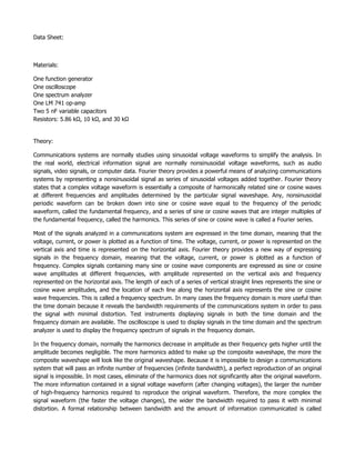
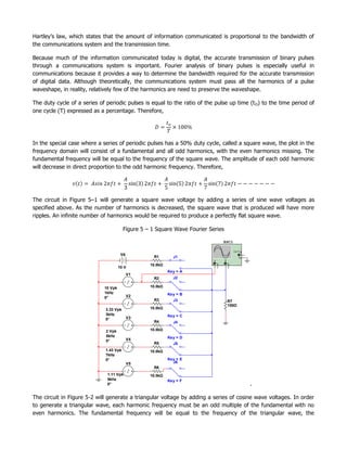
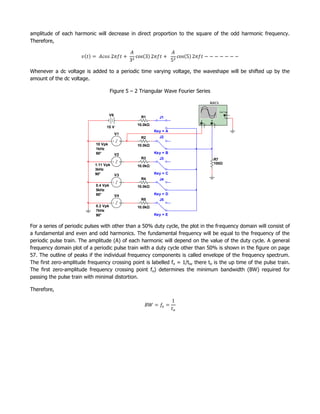
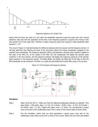
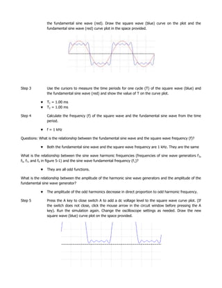
State of ICS and IoT Cyber Threat Landscape Report 2024 previewPrayukth K V
The IoT and OT threat landscape report has been prepared by the Threat Research Team at Sectrio using data from Sectrio, cyber threat intelligence farming facilities spread across over 85 cities around the world. In addition, Sectrio also runs AI-based advanced threat and payload engagement facilities that serve as sinks to attract and engage sophisticated threat actors, and newer malware including new variants and latent threats that are at an earlier stage of development.
The latest edition of the OT/ICS and IoT security Threat Landscape Report 2024 also covers:
State of global ICS asset and network exposure
Sectoral targets and attacks as well as the cost of ransom
Global APT activity, AI usage, actor and tactic profiles, and implications
Rise in volumes of AI-powered cyberattacks
Major cyber events in 2024
Malware and malicious payload trends
Cyberattack types and targets
Vulnerability exploit attempts on CVEs
Attacks on counties – USA
Expansion of bot farms – how, where, and why
In-depth analysis of the cyber threat landscape across North America, South America, Europe, APAC, and the Middle East
Why are attacks on smart factories rising?
Cyber risk predictions
Axis of attacks – Europe
Systemic attacks in the Middle East
Download the full report from here:
https://sectrio.com/resources/ot-threat-landscape-reports/sectrio-releases-ot-ics-and-iot-security-threat-landscape-report-2024/
GridMate - End to end testing is a critical piece to ensure quality and avoid...ThomasParaiso2
End to end testing is a critical piece to ensure quality and avoid regressions. In this session, we share our journey building an E2E testing pipeline for GridMate components (LWC and Aura) using Cypress, JSForce, FakerJS…
Securing your Kubernetes cluster_ a step-by-step guide to success !KatiaHIMEUR1
Today, after several years of existence, an extremely active community and an ultra-dynamic ecosystem, Kubernetes has established itself as the de facto standard in container orchestration. Thanks to a wide range of managed services, it has never been so easy to set up a ready-to-use Kubernetes cluster.
However, this ease of use means that the subject of security in Kubernetes is often left for later, or even neglected. This exposes companies to significant risks.
In this talk, I'll show you step-by-step how to secure your Kubernetes cluster for greater peace of mind and reliability.
Removing Uninteresting Bytes in Software FuzzingAftab Hussain
Imagine a world where software fuzzing, the process of mutating bytes in test seeds to uncover hidden and erroneous program behaviors, becomes faster and more effective. A lot depends on the initial seeds, which can significantly dictate the trajectory of a fuzzing campaign, particularly in terms of how long it takes to uncover interesting behaviour in your code. We introduce DIAR, a technique designed to speedup fuzzing campaigns by pinpointing and eliminating those uninteresting bytes in the seeds. Picture this: instead of wasting valuable resources on meaningless mutations in large, bloated seeds, DIAR removes the unnecessary bytes, streamlining the entire process.
In this work, we equipped AFL, a popular fuzzer, with DIAR and examined two critical Linux libraries -- Libxml's xmllint, a tool for parsing xml documents, and Binutil's readelf, an essential debugging and security analysis command-line tool used to display detailed information about ELF (Executable and Linkable Format). Our preliminary results show that AFL+DIAR does not only discover new paths more quickly but also achieves higher coverage overall. This work thus showcases how starting with lean and optimized seeds can lead to faster, more comprehensive fuzzing campaigns -- and DIAR helps you find such seeds.
- These are slides of the talk given at IEEE International Conference on Software Testing Verification and Validation Workshop, ICSTW 2022.
Observability Concepts EVERY Developer Should Know -- DeveloperWeek Europe.pdfPaige Cruz
Monitoring and observability aren’t traditionally found in software curriculums and many of us cobble this knowledge together from whatever vendor or ecosystem we were first introduced to and whatever is a part of your current company’s observability stack.
While the dev and ops silo continues to crumble….many organizations still relegate monitoring & observability as the purview of ops, infra and SRE teams. This is a mistake - achieving a highly observable system requires collaboration up and down the stack.
I, a former op, would like to extend an invitation to all application developers to join the observability party will share these foundational concepts to build on:
Generative AI Deep Dive: Advancing from Proof of Concept to ProductionAggregage
Join Maher Hanafi, VP of Engineering at Betterworks, in this new session where he'll share a practical framework to transform Gen AI prototypes into impactful products! He'll delve into the complexities of data collection and management, model selection and optimization, and ensuring security, scalability, and responsible use.
GraphSummit Singapore | The Art of the Possible with Graph - Q2 2024Neo4j
Neha Bajwa, Vice President of Product Marketing, Neo4j
Join us as we explore breakthrough innovations enabled by interconnected data and AI. Discover firsthand how organizations use relationships in data to uncover contextual insights and solve our most pressing challenges – from optimizing supply chains, detecting fraud, and improving customer experiences to accelerating drug discoveries.
In his public lecture, Christian Timmerer provides insights into the fascinating history of video streaming, starting from its humble beginnings before YouTube to the groundbreaking technologies that now dominate platforms like Netflix and ORF ON. Timmerer also presents provocative contributions of his own that have significantly influenced the industry. He concludes by looking at future challenges and invites the audience to join in a discussion.
Sudheer Mechineni, Head of Application Frameworks, Standard Chartered Bank
Discover how Standard Chartered Bank harnessed the power of Neo4j to transform complex data access challenges into a dynamic, scalable graph database solution. This keynote will cover their journey from initial adoption to deploying a fully automated, enterprise-grade causal cluster, highlighting key strategies for modelling organisational changes and ensuring robust disaster recovery. Learn how these innovations have not only enhanced Standard Chartered Bank’s data infrastructure but also positioned them as pioneers in the banking sector’s adoption of graph technology.
Smart TV Buyer Insights Survey 2024 by 91mobiles.pdf91mobiles
91mobiles recently conducted a Smart TV Buyer Insights Survey in which we asked over 3,000 respondents about the TV they own, aspects they look at on a new TV, and their TV buying preferences.
The Art of the Pitch: WordPress Relationships and SalesLaura Byrne
Clients don’t know what they don’t know. What web solutions are right for them? How does WordPress come into the picture? How do you make sure you understand scope and timeline? What do you do if sometime changes?
All these questions and more will be explored as we talk about matching clients’ needs with what your agency offers without pulling teeth or pulling your hair out. Practical tips, and strategies for successful relationship building that leads to closing the deal.
Elevating Tactical DDD Patterns Through Object CalisthenicsDorra BARTAGUIZ
After immersing yourself in the blue book and its red counterpart, attending DDD-focused conferences, and applying tactical patterns, you're left with a crucial question: How do I ensure my design is effective? Tactical patterns within Domain-Driven Design (DDD) serve as guiding principles for creating clear and manageable domain models. However, achieving success with these patterns requires additional guidance. Interestingly, we've observed that a set of constraints initially designed for training purposes remarkably aligns with effective pattern implementation, offering a more ‘mechanical’ approach. Let's explore together how Object Calisthenics can elevate the design of your tactical DDD patterns, offering concrete help for those venturing into DDD for the first time!
DevOps and Testing slides at DASA ConnectKari Kakkonen
My and Rik Marselis slides at 30.5.2024 DASA Connect conference. We discuss about what is testing, then what is agile testing and finally what is Testing in DevOps. Finally we had lovely workshop with the participants trying to find out different ways to think about quality and testing in different parts of the DevOps infinity loop.
GraphRAG is All You need? LLM & Knowledge GraphGuy Korland
Guy Korland, CEO and Co-founder of FalkorDB, will review two articles on the integration of language models with knowledge graphs.
1. Unifying Large Language Models and Knowledge Graphs: A Roadmap.
https://arxiv.org/abs/2306.08302
2. Microsoft Research's GraphRAG paper and a review paper on various uses of knowledge graphs:
https://www.microsoft.com/en-us/research/blog/graphrag-unlocking-llm-discovery-on-narrative-private-data/
Threats to mobile devices are more prevalent and increasing in scope and complexity. Users of mobile devices desire to take full advantage of the features
available on those devices, but many of the features provide convenience and capability but sacrifice security. This best practices guide outlines steps the users can take to better protect personal devices and information.
National Security Agency - NSA mobile device best practices
Pagara
1. NATIONAL COLLEGE OF SCIENCE & TECHNOLOGY
Amafel Bldg. Aguinaldo Highway Dasmariñas City, Cavite
EXPERIMENT 5
Fourier Theory – Frequency Domain and Time Domain
Pagara, Sheila Marie P. September 06, 2011
Signal Spectra and Signal Processing/BSECE 41A1 Score:
Engr. Grace Ramones
Instructor
2. Objectives:
Learn how a square wave can be produced from a series of sine waves at different frequencies and
amplitudes.
Learn how a triangular can be produced from a series of cosine waves at different frequencies and
amplitudes.
Learn about the difference between curve plots in the time domain and the frequency domain.
Examine periodic pulses with different duty cycles in the time domain and in the frequency domain.
Examine what happens to periodic pulses with different duty cycles when passed through low-pass filter
when the filter cutoff frequency is varied.
3. Sample Computation
Duty Cycle
Frequency
First zero crossing point
Bandwidth
BW =
4. Data Sheet:
Materials:
One function generator
One oscilloscope
One spectrum analyzer
One LM 741 op-amp
Two 5 nF variable capacitors
Resistors: 5.86 kΩ, 10 kΩ, and 30 kΩ
Theory:
Communications systems are normally studies using sinusoidal voltage waveforms to simplify the analysis. In
the real world, electrical information signal are normally nonsinusoidal voltage waveforms, such as audio
signals, video signals, or computer data. Fourier theory provides a powerful means of analyzing communications
systems by representing a nonsinusoidal signal as series of sinusoidal voltages added together. Fourier theory
states that a complex voltage waveform is essentially a composite of harmonically related sine or cosine waves
at different frequencies and amplitudes determined by the particular signal waveshape. Any, nonsinusoidal
periodic waveform can be broken down into sine or cosine wave equal to the frequency of the periodic
waveform, called the fundamental frequency, and a series of sine or cosine waves that are integer multiples of
the fundamental frequency, called the harmonics. This series of sine or cosine wave is called a Fourier series.
Most of the signals analyzed in a communications system are expressed in the time domain, meaning that the
voltage, current, or power is plotted as a function of time. The voltage, current, or power is represented on the
vertical axis and time is represented on the horizontal axis. Fourier theory provides a new way of expressing
signals in the frequency domain, meaning that the voltage, current, or power is plotted as a function of
frequency. Complex signals containing many sine or cosine wave components are expressed as sine or cosine
wave amplitudes at different frequencies, with amplitude represented on the vertical axis and frequency
represented on the horizontal axis. The length of each of a series of vertical straight lines represents the sine or
cosine wave amplitudes, and the location of each line along the horizontal axis represents the sine or cosine
wave frequencies. This is called a frequency spectrum. In many cases the frequency domain is more useful than
the time domain because it reveals the bandwidth requirements of the communications system in order to pass
the signal with minimal distortion. Test instruments displaying signals in both the time domain and the
frequency domain are available. The oscilloscope is used to display signals in the time domain and the spectrum
analyzer is used to display the frequency spectrum of signals in the frequency domain.
In the frequency domain, normally the harmonics decrease in amplitude as their frequency gets higher until the
amplitude becomes negligible. The more harmonics added to make up the composite waveshape, the more the
composite waveshape will look like the original waveshape. Because it is impossible to design a communications
system that will pass an infinite number of frequencies (infinite bandwidth), a perfect reproduction of an original
signal is impossible. In most cases, eliminate of the harmonics does not significantly alter the original waveform.
The more information contained in a signal voltage waveform (after changing voltages), the larger the number
of high-frequency harmonics required to reproduce the original waveform. Therefore, the more complex the
signal waveform (the faster the voltage changes), the wider the bandwidth required to pass it with minimal
distortion. A formal relationship between bandwidth and the amount of information communicated is called
5. Hartley’s law, which states that the amount of information communicated is proportional to the bandwidth of
the communications system and the transmission time.
Because much of the information communicated today is digital, the accurate transmission of binary pulses
through a communications system is important. Fourier analysis of binary pulses is especially useful in
communications because it provides a way to determine the bandwidth required for the accurate transmission
of digital data. Although theoretically, the communications system must pass all the harmonics of a pulse
waveshape, in reality, relatively few of the harmonics are need to preserve the waveshape.
The duty cycle of a series of periodic pulses is equal to the ratio of the pulse up time (t O) to the time period of
one cycle (T) expressed as a percentage. Therefore,
In the special case where a series of periodic pulses has a 50% duty cycle, called a square wave, the plot in the
frequency domain will consist of a fundamental and all odd harmonics, with the even harmonics missing. The
fundamental frequency will be equal to the frequency of the square wave. The amplitude of each odd harmonic
will decrease in direct proportion to the odd harmonic frequency. Therefore,
The circuit in Figure 5–1 will generate a square wave voltage by adding a series of sine wave voltages as
specified above. As the number of harmonics is decreased, the square wave that is produced will have more
ripples. An infinite number of harmonics would be required to produce a perfectly flat square wave.
Figure 5 – 1 Square Wave Fourier Series
XSC1
Ext T rig
V6 +
R1 J1 _
A B
10.0kΩ + _ + _
10 V
Key = A
V1
R2 J2
10 Vpk 10.0kΩ
1kHz Key = B
0° V2
R3 J3 4
155
0
8
160
14
13
12 R7
109
02
3 100Ω
3.33 Vpk 10.0kΩ
3kHz Key = C
0° V3
R4 J4
2 Vpk 10.0kΩ
5kHz Key = D
0° V4
R5 J5
1.43 Vpk 10.0kΩ
7kHz
0° Key = E
V5 J6
R6
1.11 Vpk 10.0kΩ
9kHz Key = F
0° .
The circuit in Figure 5-2 will generate a triangular voltage by adding a series of cosine wave voltages. In order
to generate a triangular wave, each harmonic frequency must be an odd multiple of the fundamental with no
even harmonics. The fundamental frequency will be equal to the frequency of the triangular wave, the
6. amplitude of each harmonic will decrease in direct proportion to the square of the odd harmonic frequency.
Therefore,
Whenever a dc voltage is added to a periodic time varying voltage, the waveshape will be shifted up by the
amount of the dc voltage.
Figure 5 – 2 Triangular Wave Fourier Series
XSC1
Ext T rig
V6 +
R1 J1 _
A B
10.0kΩ + _ + _
15 V
Key = A
V1
R2 J2
10 Vpk 10.0kΩ
1kHz
90° V2 Key = B
R3 J3 13
12
1
2
3
4
5
8
9
11
0 R7
6
0
1.11 Vpk 100Ω
10.0kΩ
3kHz
90° V3 Key = C
R4 J4
0.4 Vpk 10.0kΩ
5kHz
90° V4 Key = D
R5 J5
0.2 Vpk 10.0kΩ
7kHz
90° Key = E
For a series of periodic pulses with other than a 50% duty cycle, the plot in the frequency domain will consist of
a fundamental and even and odd harmonics. The fundamental frequency will be equal to the frequency of the
periodic pulse train. The amplitude (A) of each harmonic will depend on the value of the duty cycle. A general
frequency domain plot of a periodic pulse train with a duty cycle other than 50% is shown in the figure on page
57. The outline of peaks if the individual frequency components is called envelope of the frequency spectrum.
The first zero-amplitude frequency crossing point is labelled fo = 1/to, there to is the up time of the pulse train.
The first zero-amplitude frequency crossing point fo) determines the minimum bandwidth (BW) required for
passing the pulse train with minimal distortion.
Therefore,
7. A
f=1/to f
2/to
Frequency Spectrum of a Pulse Train
Notice than the lower the value of t o the wider the bandwidth required to pass the pulse train with minimal
distortion. Also note that the separation of the lines in the frequency spectrum is equal to the inverse of the
time period (1/T) of the pulse train. Therefore a higher frequency pulse train requires a wider bandwidth (BW)
because f = 1/T
The circuit in Figure 5-3 will demonstrate the difference between the time domain and the frequency domain. It
will also determine how filtering out some of the harmonics effects the output waveshape compared to the
original3 input waveshape. The frequency generator (XFG1) will generate a periodic pulse waveform applied to
the input of the filter (5). At the output of the filter (70, the oscilloscope will display the periodic pulse
waveform in the time domain, and the spectrum analyzer will display the frequency spectrum of the periodic
pulse waveform in the frequency domain. The Bode plotter will display the Bode plot of the filter so that the
filter bandwidth can be measured. The filter is a 2-pole low-pass Butterworth active filter using a 741 op-amp.
Figure 5-3 Time Domain and Frequency Domain
XFG1
XSC1
C1 XSA1
Ext T rig
+
2.5nF 50% _
Key=A A
_
B
_
IN T
+ +
R1 R2 741
30kΩ 30kΩ
42
OPAMP_3T_VIRTUAL
0
6
0
31
R3
C2 R4
5.56kΩ
10kΩ
XBP1
2.5nF 50%
Key=A
R5 IN OUT
10kΩ
Procedure:
Step 1 Open circuit file FIG 5-1. Make sure that the following oscilloscope settings are selected: Time
base (Scale = 200 µs/Div, Xpos = 0, Y/t), Ch A (Scale = 5V/Div, Ypos = 0, DC), Ch B (Scale =
50 mV/Div, Ypos = 0, DC), Trigger (Pos edge, Level = 0, Auto). You will generate a square
wave curve plot on the oscilloscope screen from a series of sine waves called a Fourier series.
Step 2 Run the simulation. Notice that you have generated a square wave curve plot on the
oscilloscope screen (blue curve) from a series of sine waves. Notice that you have also plotted
8. the fundamental sine wave (red). Draw the square wave (blue) curve on the plot and the
fundamental sine wave (red) curve plot in the space provided.
Step 3 Use the cursors to measure the time periods for one cycle (T) of the square wave (blue) and
the fundamental sine wave (red) and show the value of T on the curve plot.
T1 = 1.00 ms
T2 = 1.00 ms
Step 4 Calculate the frequency (f) of the square wave and the fundamental sine wave from the time
period.
f = 1 kHz
Questions: What is the relationship between the fundamental sine wave and the square wave frequency (f)?
Both the fundamental sine wave and the square wave frequency are 1 kHz. They are the same
What is the relationship between the sine wave harmonic frequencies (frequencies of sine wave generators f 3,
f5, f7, and f9 in figure 5-1) and the sine wave fundamental frequency (f 1)?
They are all odd functions.
What is the relationship between the amplitude of the harmonic sine wave generators and the amplitude of the
fundamental sine wave generator?
The amplitude of the odd harmonics decrease in direct proportion to odd harmonic frequency.
Step 5 Press the A key to close switch A to add a dc voltage level to the square wave curve plot. (If
the switch does not close, click the mouse arrow in the circuit window before pressing the A
key). Run the simulation again. Change the oscilloscope settings as needed. Draw the new
square wave (blue) curve plot on the space provided.
9. Question: What happened to the square wave curve plot? Explain why.
The waveshape moved upwards because of the additional dc voltage.
Step 6 Press the F and E keys to open the switches F and E to eliminate the ninth and seventh
harmonic sine waves. Run the simulation again. Draw the new curve plot (blue) in the space
provided. Note any change on the graph.
Step 7 Press the D key to open the switch D to eliminate the fifth harmonics sine wave. Run the
simulation again. Draw the new curve plot (blue) in the space provided. Note any change on
the graph.
Step 8 Press the C key to open switch C and eliminate the third harmonic sine wave. Run the
simulation again.
Question: What happened to the square wave curve plot? Explain.
It became sinusoidal. Because the sine wave harmonics are missing, the waveshape became
the sine wave fundamental
Step 9 Open circuit file FIG 5-2. Make sure that the following oscilloscope settings are selected: Time
base (Scale = 200 µs/Div, Xpos = 0, Y/t), Ch A (Scale = 5V/Div, Ypos = 0, DC), Ch B (Scale =
100 mV/Div, Ypos = 0, DC), Trigger (Pos edge, Level = 0, Auto). You will generate a triangular
wave curve plot on the oscilloscope screen from a series of sine waves called a Fourier series.
Step 10 Run the simulation. Notice that you have generated a triangular wave curve plot on the
oscilloscope screen (blue curve) from the series of cosine waves. Notice that you have also
plotted the fundamental cosine wave (red). Draw the triangular wave (blue) curve plot and the
fundamental cosine wave (red) curve plot in the space provided.
10. Step 11 Use the cursors to measure the time period for one cycle (T) of the triangular wave (blue) and
the fundamental (red), and show the value of T on the curve plot.
T1 = 1.00 ms
T2 = 1.00 ms
Step 12 Calculate the frequency (f) of the triangular wave from the time period (T).
f = 1 kHz
Questions: What is the relationship between the fundamental frequency and the triangular wave frequency?
The frequencies are the same.
What is the relationship between the harmonic frequencies (frequencies of generators f 3, f5, and f7 in figure 5-2)
and the fundamental frequency (f1)?
The frequencies are all odd functions.
What is the relationship between the amplitude of the harmonic generators and the amplitude of the
fundamental generator?
The amplitude of the odd harmonics decrease in direct proportion to odd harmonic frequency.
Step 13 Press the A key to close switch A to add a dc voltage level to the triangular wave curve plot.
Run the simulation again. Draw the new triangular wave (blue) curve plot on the space
provided.
Question: What happened to the triangular wave curve plot? Explain.
The waveshape moved upwards because of the additional dc voltage.
11. Step 14 Press the E and D keys to open switches E and D to eliminate the seventh and fifth harmonic
sine waves. Run the simulation again. Draw the new curve plot (blue) in the space provided.
Note any change on the graph.
Step 15 Press the C key to open the switch C to eliminate the third harmonics sine wave. Run the
simulation again.
Question: What happened to the triangular wave curve plot? Explain.
it became sinusoidal. Bhe sine wave harmonics are missing, the waveshape became the sine
wave fundamental
Step 16 Open circuit FIG 5-3. Make sure that following function generator settings are selected: Square
wave, Freq = 1 kHz, Duty cycle = 50%, Ampl – 2.5 V, Offset = 2.5 V. Make sure that the
following oscilloscope settings are selected: Time base (Scale = 500 µs/Div, Xpos = 0, Y/T), Ch
A (Scale = 5 V/Div, Ypos = 0, DC), Ch B (Scale = 5 V/Div, Ypos = 0, DC), Trigger (pos edge,
Level = 0, Auto). You will plot a square wave in the time domain at the input and output of a
two-pole low-pass Butterworth filter.
Step 17 Bring down the oscilloscope enlargement and run the simulation to one full screen display, then
pause the simulation. Notice that you are displaying square wave curve plot in the time domain
(voltage as a function of time). The red curve plot is the filter input (5) and the blue curve plot
is the filter output (7)
Question: Are the filter input (red) and the output (blue) plots the same shape disregarding any amplitude
differences?
Yes.
Step 18 Use the cursor to measure the time period (T) and the time (fo) of the input curve plot (red)
and record the values.
T= 1 ms to = 500.477µs
Step 19 Calculate the pulse duty cycle (D) from the to and T
D = 50.07%.
Question: How did your calculated duty cycle compare with the duty cycle setting on the function generator?
They have difference of 0.07%.
12. Step 20 Bring down the Bode plotter enlargement to display the Bode plot of the filter. Make sure that
the following Bode plotter settings are selected; Magnitude, Vertical (Log, F = 10 dB, I = -40
dB), Horizontal (Log, F = 200 kHz, I = 100 Hz). Run the simulation to completion. Use the
cursor to measure the cutoff frequency (fC) of the low-pass filter and record the value.
fC = 21.197
Step 21 Bring down the analyzer enlargement. Make sure that the following spectrum analyzer settings
are selected: Freq (Start = 0 kHz, Center = 5 kHz, End = 10 kHz), Ampl (Lin, Range = 1 V/Div),
Res = 50 Hz. Run the simulation until the Resolution frequencies match, then pause the
simulation. Notice that you have displayed the filter output square wave frequency spectrum in
the frequency domain, use the cursor to measure the amplitude of the fundamental and each
harmonic to the ninth and record your answers in table 5-1.
Table 5-1
Frequency (kHz) Amplitude
f1 1 5.048 V
f2 2 11.717 µV
f3 3 1.683 V
f4 4 15.533 µV
f5 5 1.008 V
f6 6 20.326 µV
f7 7 713.390 mV
f8 8 25.452 µV
f9 9 552.582 mV
Questions: What conclusion can you draw about the difference between the even and odd harmonics for a
square wave with the duty cycle (D) calculated in Step 19?
The frequency domain consists of a fundamental and odd harmonics while the even harmonics
are almost zero.
What conclusions can you draw about the amplitude of each odd harmonic compared to the fundamental for a
square wave with the duty cycle (D) calculated in Step 19?
The amplitude of each odd harmonic decreases as the fundamental frequency for a square
wave.
Was this frequency spectrum what you expected for a square wave with the duty cycle (D) calculated in Step
19?
Yes.
Based on the filter cutoff frequency (f C) measured in Step 20, how many of the square wave harmonics would
you expect to be passed by this filter? Based on this answer, would you expect much distortion of the input
square wave at the filter? Did your answer in Step 17 verify this conclusion?
There are square waves. Yes, because the more number of harmonics square wave the more
distortion in the input square wave.
13. Step 22 Adjust both filter capacitors (C) to 50% (2.5 nF) each. (If the capacitors won’t change, click the
mouse arrow in the circuit window). Bring down the oscilloscope enlargement and run the
simulation to one full screen display, then pause the simulation. The red curve plot is the filter
input and the blue curve plot is the filter output.
Question: Are the filter input (red) and output (blue) curve plots the same shape, disregarding any amplitude
differences?
No.
Step 23 Bring down the Bode plotter enlargement to display the Bode plot of the filter. Use the cursor to
measure the cutoff frequency (Fc of the low-pass filter and record the value.
fc = 2.12 kHz
Step 24 Bring down the spectrum analyzer enlargement to display the filter output frequency spectrum
in the frequency domain, Run the simulation until the Resolution Frequencies match, then
pause the simulation. Use cursor to measure the amplitude of the fundamental and each
harmonic to the ninth and record your answers in Table 5-2.
Table 5-2
Frequency (kHz) Amplitude
f1 1 4.4928 V
f2 2 4.44397µV
f3 3 792.585 mV
f4 4 323.075 µV
f5 5 178.663mV
f6 6 224.681 µV
f7 7 65.766 mV
f8 8 172.430 µV
f9 9 30.959 mV
Questions: How did the amplitude of each harmonic in Table 5-2 compare with the values in Table 5-1?
Compare with the previous table, the value of the amplitude of the harmonics is lower.
Based on the filter cutoff frequency (f c), how many of the square wave harmonics should be passed by this
filter? Based on this answer, would you expect much distortion of the input square wave at the filter output?
Did your answer in Step 22 verify this conclusion?
Based on the fc, there should be less than 5 square wave harmonics.. Yes, there have much
distortion in the input square wave at the filter output.
Step 25 Change the both capacitor (C) back to 5% (0.25 nF). Change the duty cycle to 20% on the
function generator. Bring down the oscilloscope enlargement and run the simulation to one full
screen display, then pause the simulation. Notice that you have displayed a pulse curve plot on
the oscilloscope in the time domain (voltage as a function of time). The red curve plot is the
filter input and the blue curve plot is the filter output.
Question: Are the filter input (red) and the output (blue) curve plots the same shape, disregarding any
amplitude differences?
14. Yes.
Step 26 Use the cursors to measure the time period (T) and the up time (t o) of the input curve plot
(red) and record the values.
T= 1 ms to =
Step 27 Calculate the pulse duty cycle (D) from the to and T.
D = 19.82%
Question: How did your calculated duty cycle compare with the duty cycle setting on the function generator?
The calculated duty cycle compare with the duty cycle setting on the function generator are
almost the same. Their difference is only 0.18%
Step 28 Bring down the Bode plotter enlargement to display the Bode plot of the filter. Use the cursor to
measure the cutoff frequency (fC) of the low-pass filter and record the value.
fC = 21.197 kHz
Step 29 Bring down the spectrum analyzer enlargement to display the filter output frequency spectrum
in the frequency domain. Run the simulation until the Resolution Frequencies match, then
pause the simulation. Draw the frequency plot in the space provided. Also draw the envelope of
the frequency spectrum.
5.041 kHz
Question: Is this the frequency spectrum you expected for a square wave with duty cycle less than 50%?
Yes.
Step 30 Use the cursor to measure the frequency of the first zero crossing point (f o) of the spectrum
envelope and record your answer on the graph.
fo = 5.041 kHz
Step 31 Based on the value of the to measured in Step 26, calculate the expected first zero crossing
point (fo) of the spectrum envelope.
fo = 5.045 kHz
15. Question: How did your calculated value of fo compare the measured value on the curve plot?
They have a difference of 0.004 Hz
Step 32 Based on the value of fo, calculate the minimum bandwidth (BW) required for the filter to pass
the input pulse waveshape with minimal distortion.
BW = 5.045 kHz
Question: Based on this answer and the cutoff frequency (f c) of the low-pass filter measure in Step 28, would
you expect much distortion of the input square wave at the filter output? Did your answer in Step 25 verify this
conclusion?
No, there is no much distortion of the input square wave at the filter output. the higher the
bandwidth, the lesser the distortion formed.
Step 33 Adjust the filter capacitors (C) to 50% (2.5 nF) each. Bring down the oscilloscope enlargement
and run the simulation to one full screen display, then pause the simulation. The red curve plot
is the filter input and the blue curve plot is the filter output.
Question: Are the filter input (red) and the output (blue) curve plots the same shape, disregarding any
amplitude differences?
No.
Step 34 Bring down the Bode plotter enlargement to display the Bode plot of the filter. Use the cursor to
measure the cutoff frequency (fc) of the low-pass filter and record the value.
fc = 4.239 kHz
Questions: Was the cutoff frequency (fc) less than or greater than the minimum bandwidth (BW) required to
pass the input waveshape with minimal distortion as determined in Step 32?
The cutoff frequency (fc) is greater than the minimum bandwidth (BW).
Based on this answer, would you expect much distortion of the input pulse waveshape at the filter output? Did
your answer in Step 33 verify this conclusion?
No, there will have much distortion.
Step 35 Bring down the spectrum analyzer enlargement to display the filter output frequency spectrum in the
frequency domain. Run the simulation until the Resolution Frequencies match, then pause the simulation.
Question: What is the difference between this frequency plot and the frequency plot in Step 29?
The amplitude in the frequency plot is much lower.
16. Conclusion:
In observing the behaviour of waveshape, I can say that a nonsinusoidal wave can be a series of sine
or cosine wave. When a dc voltage source was added, the curve will move upwards. The more the harmonics
added to the fundamental sine wave the more the curve will be a complex wave. Meaning, the more the
harmonics added, the more the wave will become nonsinusoidal wave. The fundamental frequency will be equal
to the frequency of the triangular wave. In square wave the amplitude of each harmonic will decrease in direct
proportion to the odd harmonic frequency. While in triangular wave, the amplitude of each harmonic will
decrease in direct proportion to the square of the odd harmonic frequency. 50% duty cycle will consist of only
odd function while the duty cycle other than 50%, the plot in the frequency domain will consist even and odd
harmonics and the fundamental wave. The lower the increment the more the output will be like the input.