Downloaded 236 times


![12
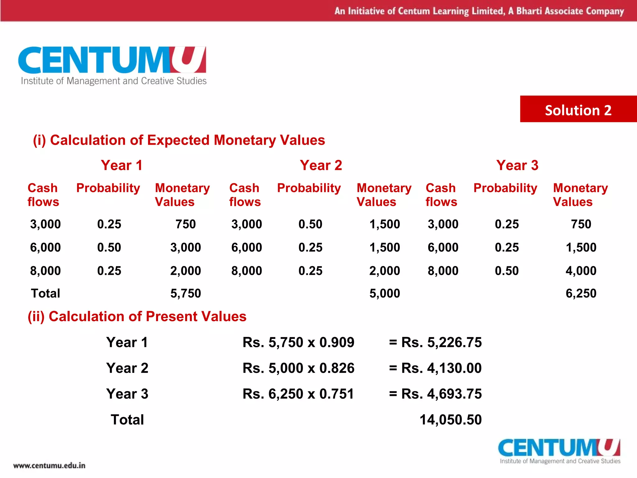
The expected returns RA and RB are just the possible returns multiplied by the
associated probabilities as follows:
RA = (0.20 x – 0.15) + (0.50 x 0.20) + (0.30 x 0.60)
= 25 %
RB = (0.20 x 0.20) + (0.50 x 0.30) + (0.30 x 0.40)
= 31 %
The standard deviations can now be calculated as follows:
σA = [0.20 (- 0.15 – 0.25)2
+ 0.50 (0.20 – 0.25)2
+ 0.30 (0.60 – 0.25)2
]1/2
= (0.0700)1/2
= 26.46 %
σB = [0.20 (0.20 – 0.31)2
+ 0.50 (0.30 – 0.31)2
+ 0.30 (0.40 – 0.31)2
]1/2
= (0.0049)1/2
= 7 %
Solution 3
The expected return and standard deviation of the portfolio of the
investor are:
Expected return = (0.75 x 0.25) + (0.25 x 0.31) = 26.5 %
Continued….](https://image.slidesharecdn.com/sensitivityscenarioanalysis-12897113987437-phpapp01/75/Sensitivity-amp-Scenario-Analysis-12-2048.jpg)
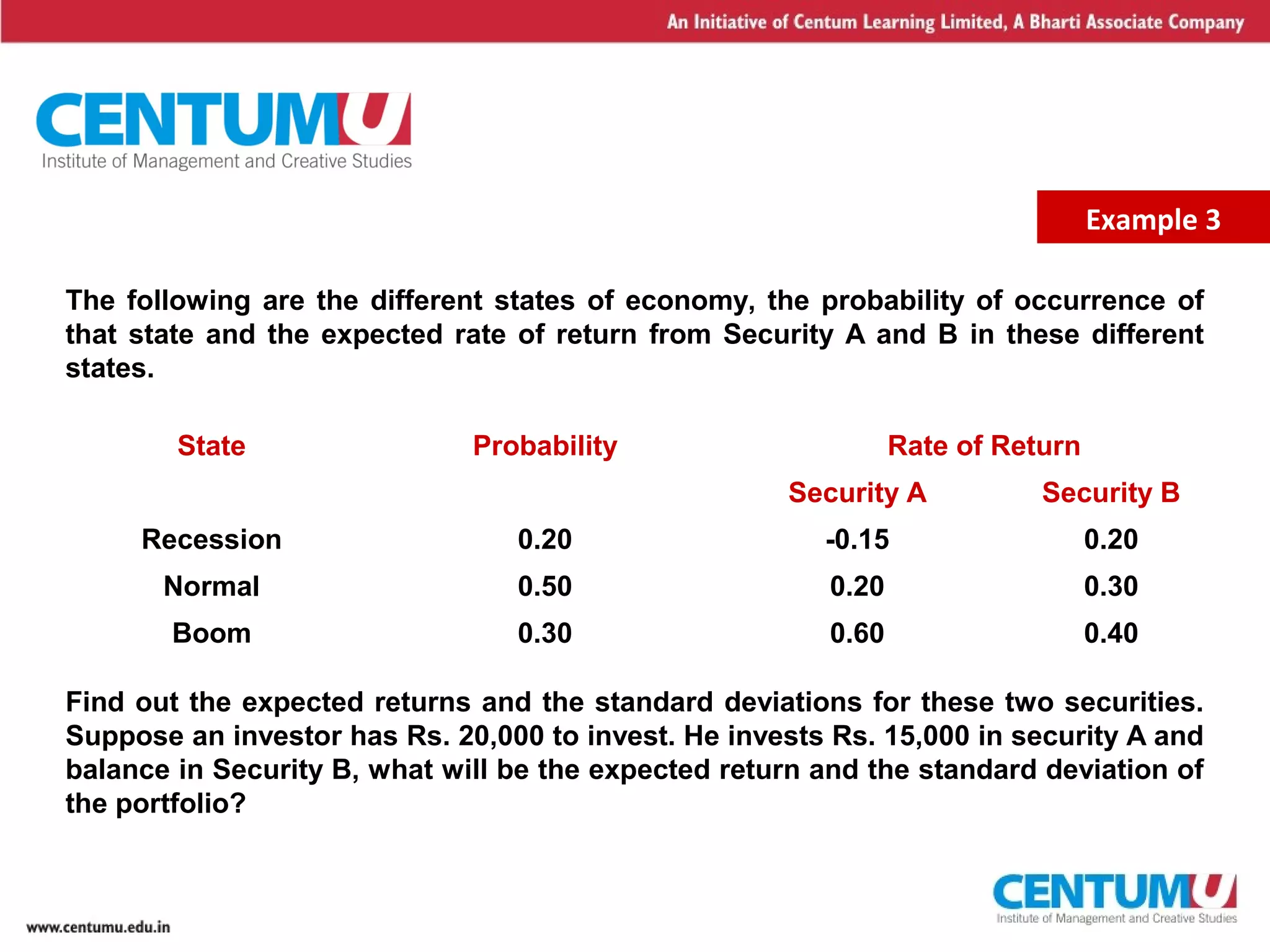
![13
Solution 3
Note: As the investor is investing Rs. 15,000 in A and Rs. 5000 in B, his portfolio will
consist of 0.75 of A and 0. 25 of B.
State Probability Expected Return
Recession 0.20 (0.75 x – 0.15) + (0.25 x 0.20) = - 0.0625
Normal 0.50 (0.75 x 0.20) + (0.25 x 0.30) = 0.2250
Boom 0.30 (0.75 x 0.60) + (0.25 x 0.40) = 0.5500
Expected Return = (0.20 x – 0.0625) + (0.50 x 0.2250) + (0.30 x 0.5500)
= 26.5 %
The standard deviation of the portfolio is:
σ = [0.20 (- 0.0625-0.265)2
+ 0.50(0.225 – 0.265)2
+ 0.30(0.550 – 0.265)2
]1/2
= [0.0466]1/2
= 21.59%
Alternatively, expected return and standard deviation can also be found by:](https://image.slidesharecdn.com/sensitivityscenarioanalysis-12897113987437-phpapp01/75/Sensitivity-amp-Scenario-Analysis-13-2048.jpg)


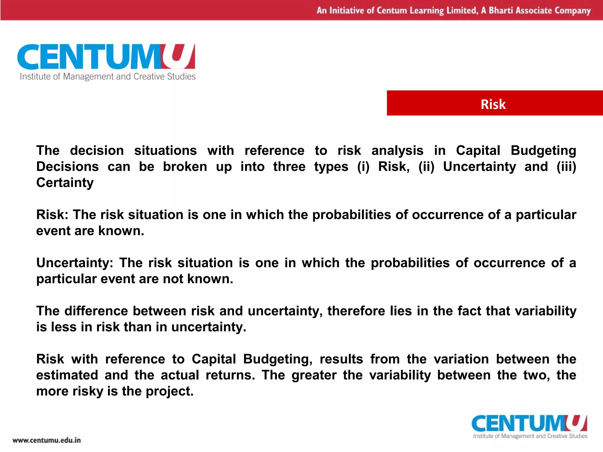
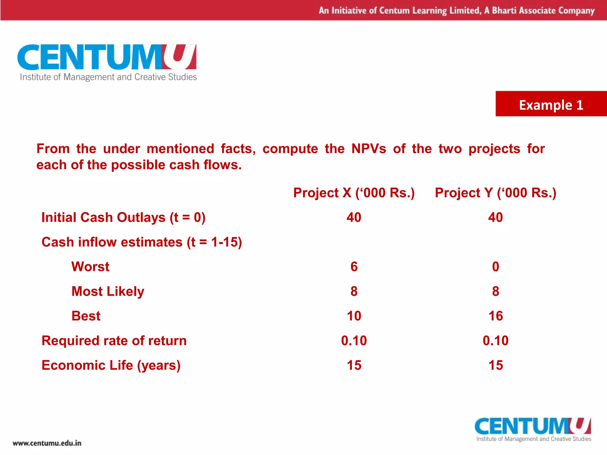
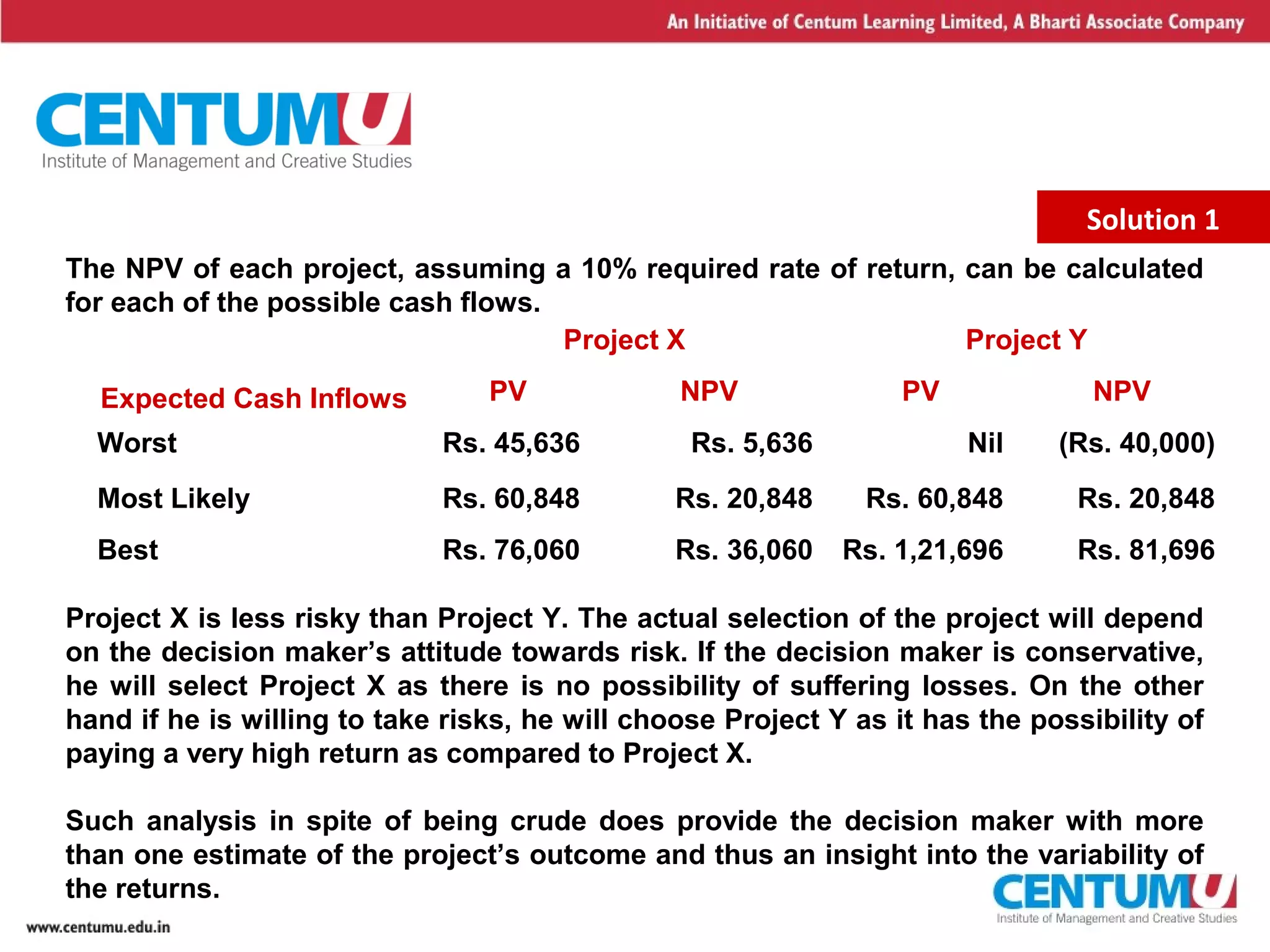
The document discusses various techniques for analyzing risk in capital budgeting decisions: - Risk refers to situations where probabilities of outcomes are known, while uncertainty refers to unknown probabilities. Risk is less variable than uncertainty. - Sensitivity analysis determines how sensitive NPV is to changes in variable assumptions by changing one variable at a time. - Scenario analysis considers multiple scenarios and their probabilities to arrive at an expected NPV. - Examples demonstrate calculating NPVs and expected returns for projects with different potential cash flows and probabilities. This provides insight into variability and risk.