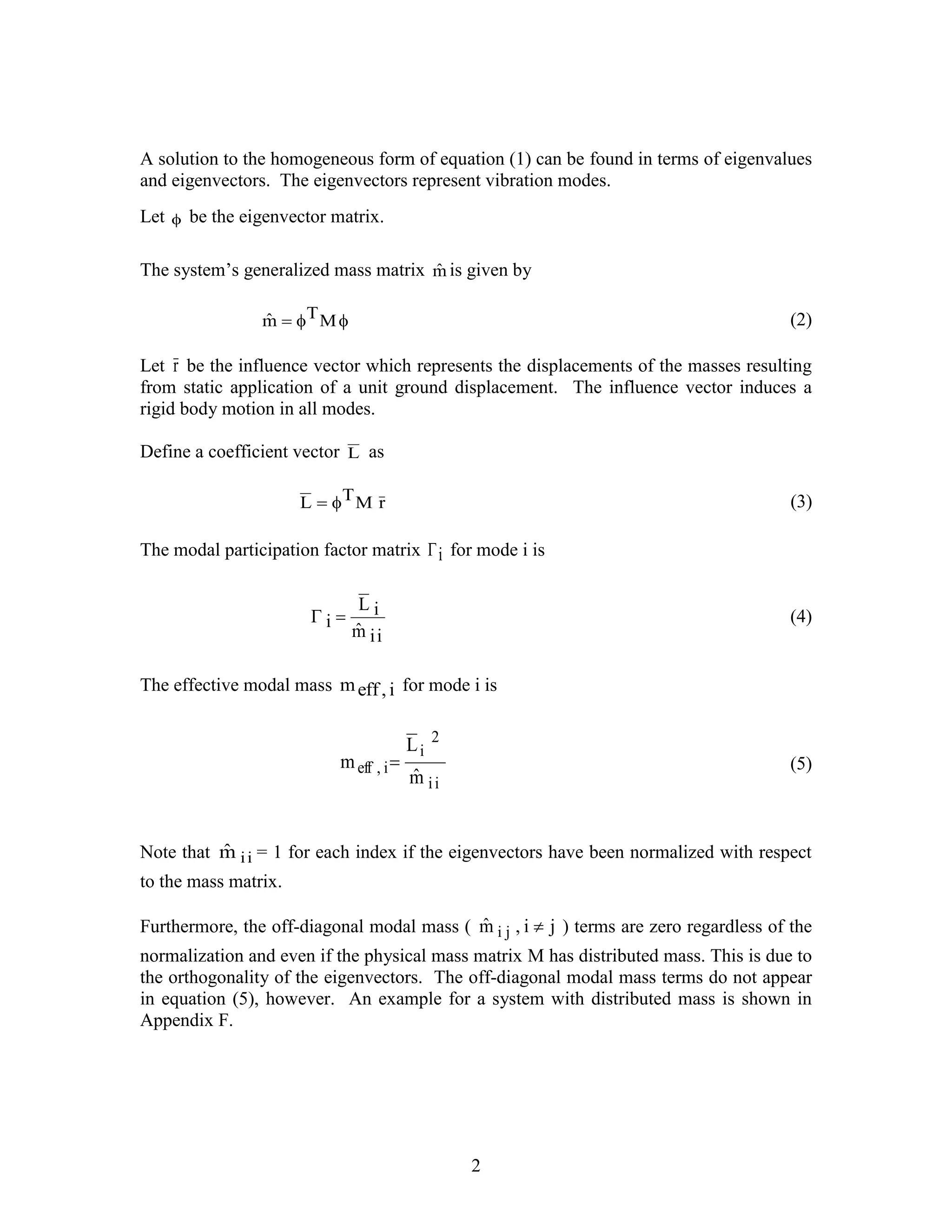
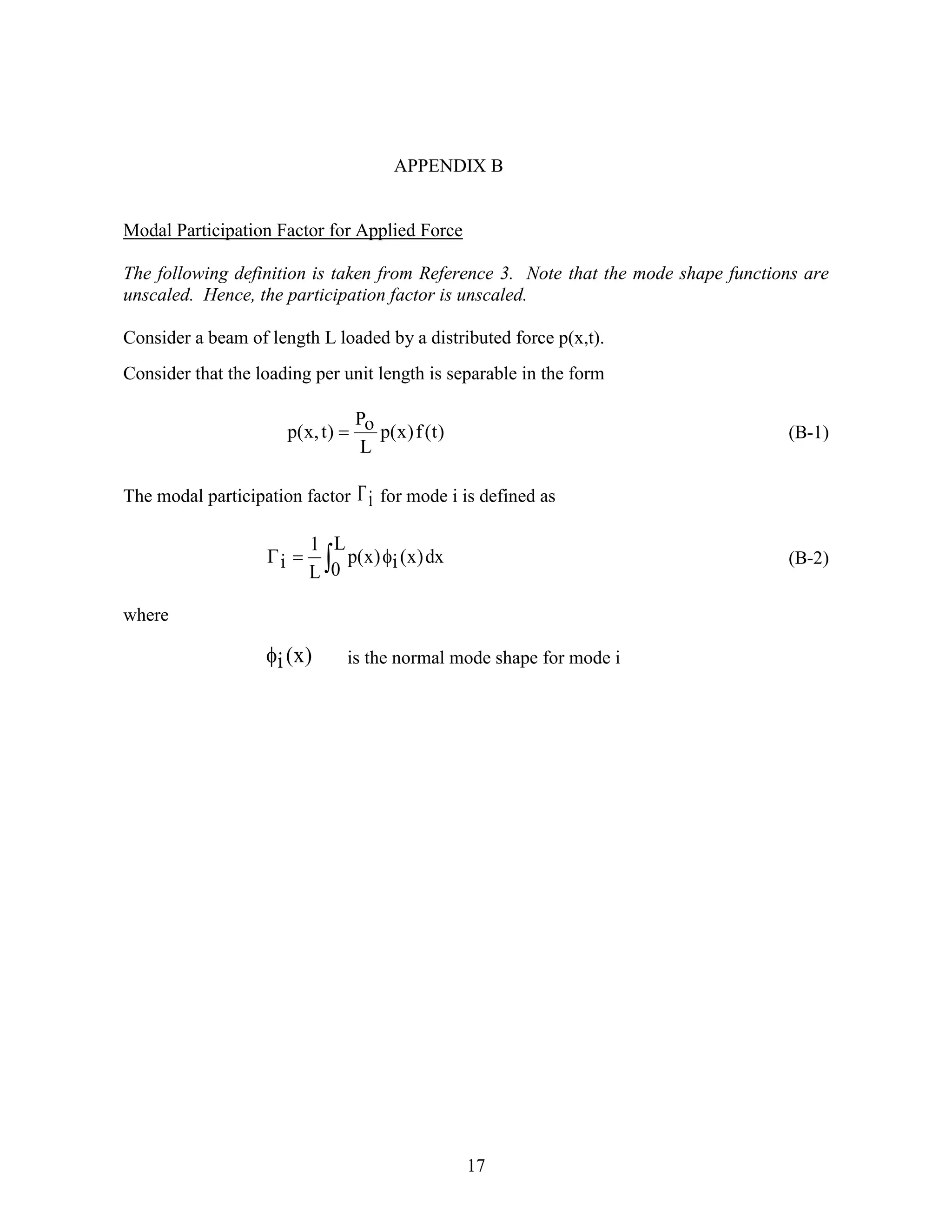
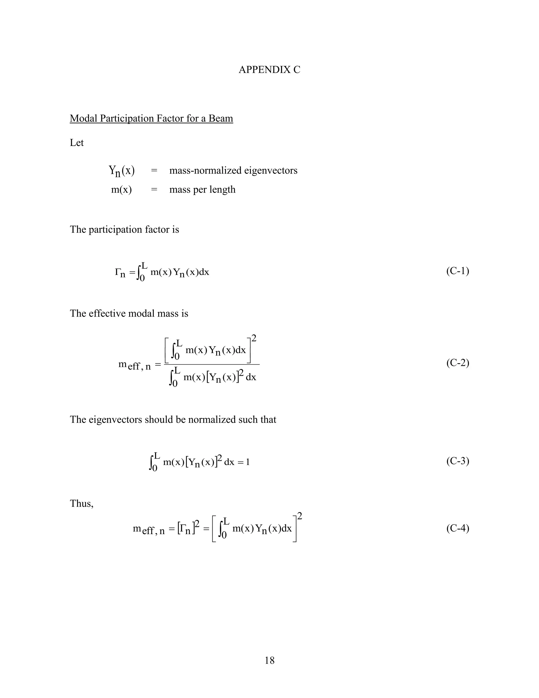
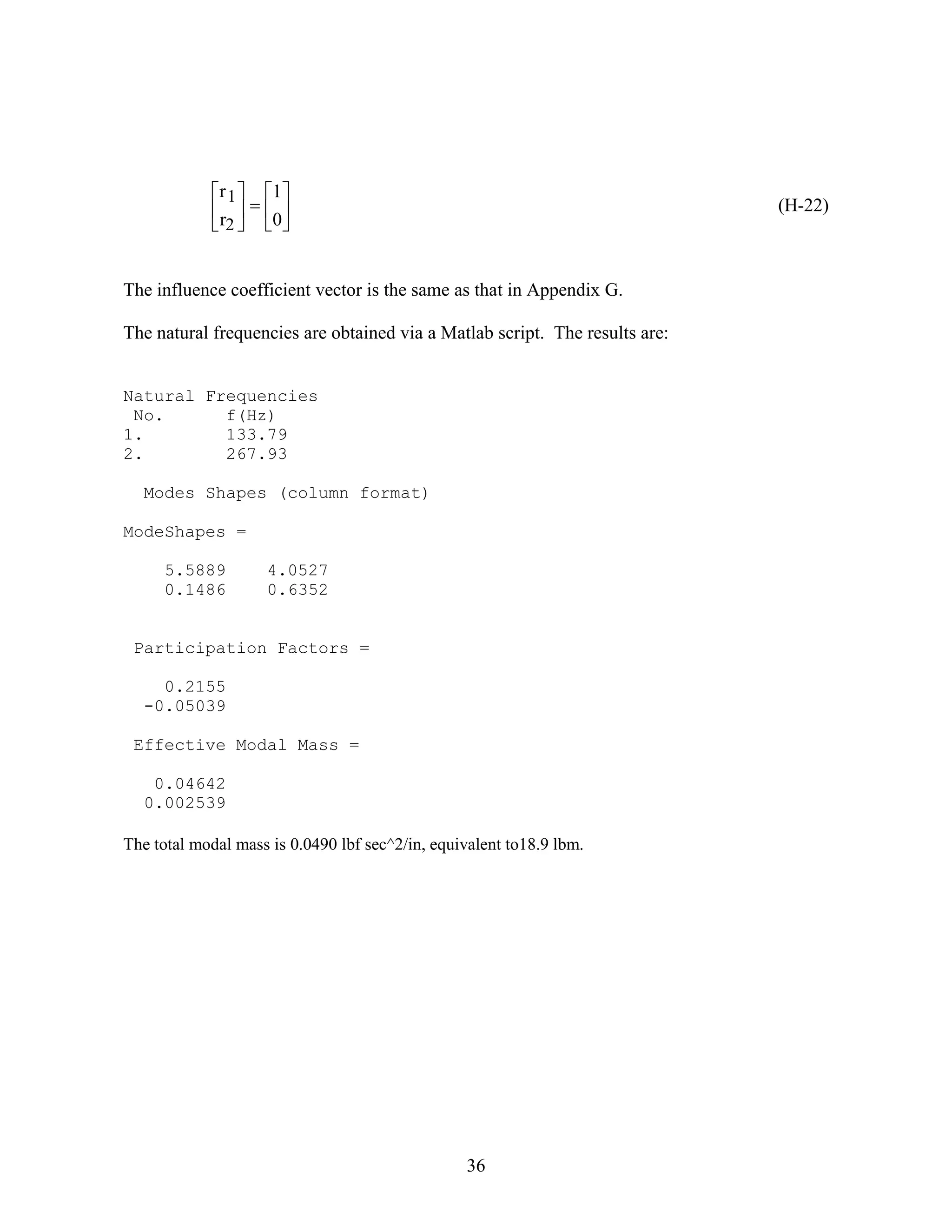
1) The document discusses effective modal mass and modal participation factors, which are methods for determining how readily a vibration mode of a system can be excited. Modes with higher effective masses can be more easily excited by base excitation.
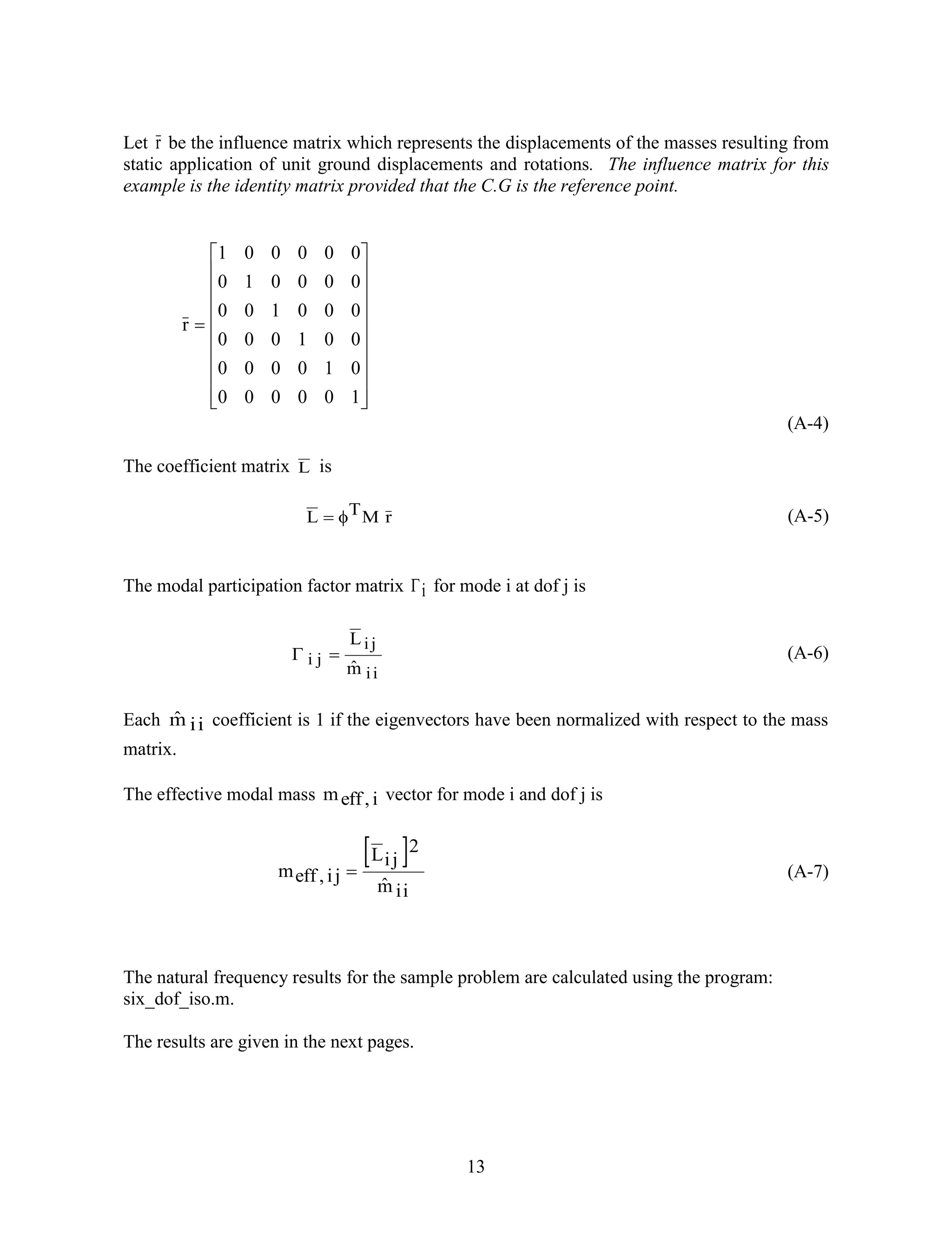
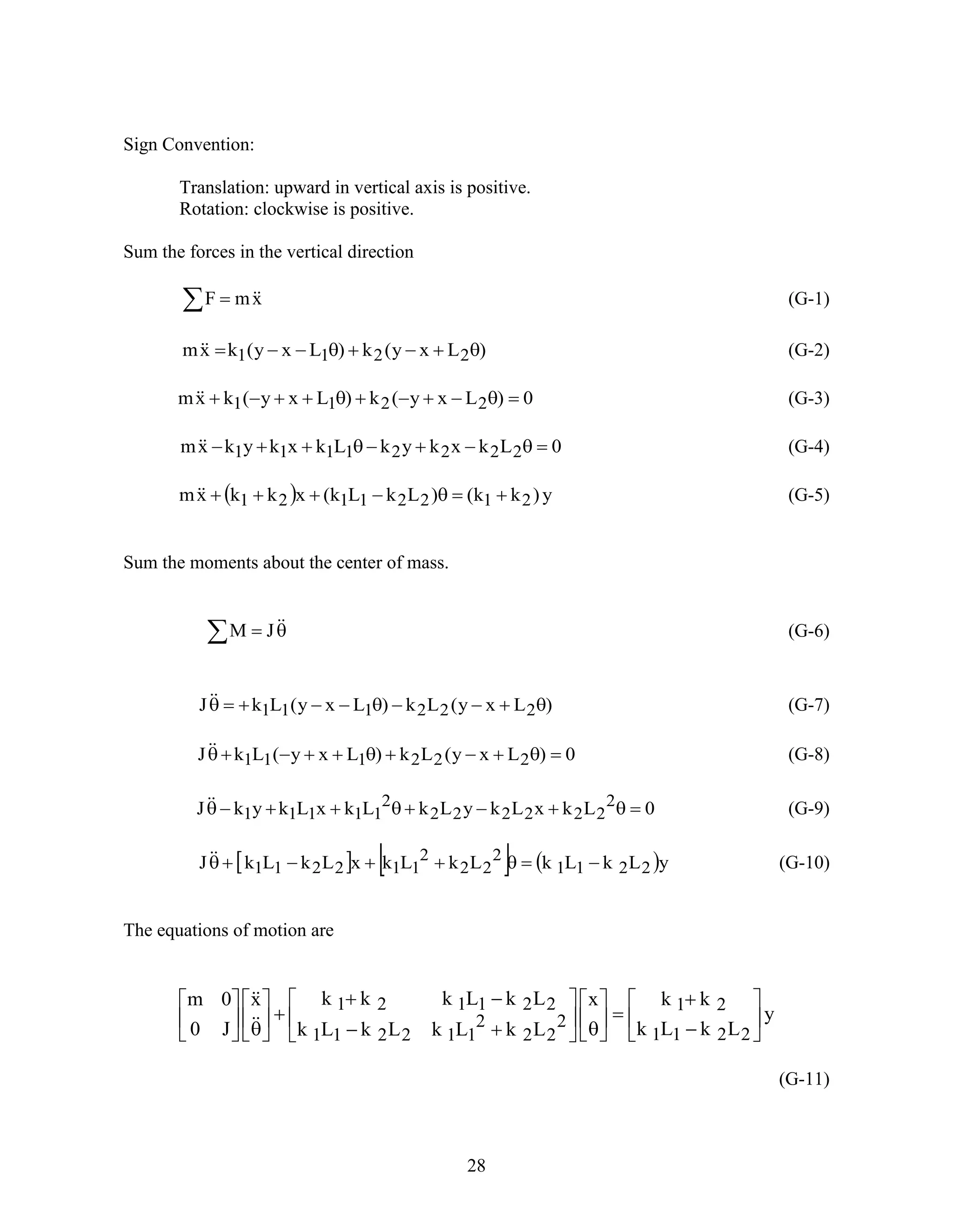
2) It provides definitions and equations for calculating effective modal mass and modal participation factors. These include the mass matrix, stiffness matrix, eigenvectors, influence vector, coefficient vector, modal participation factor matrix, and effective modal mass.
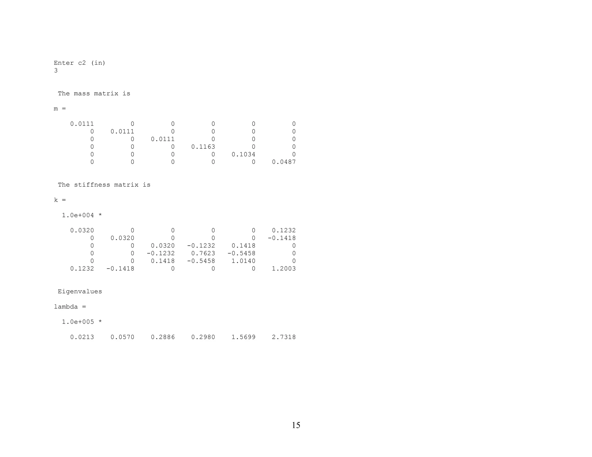
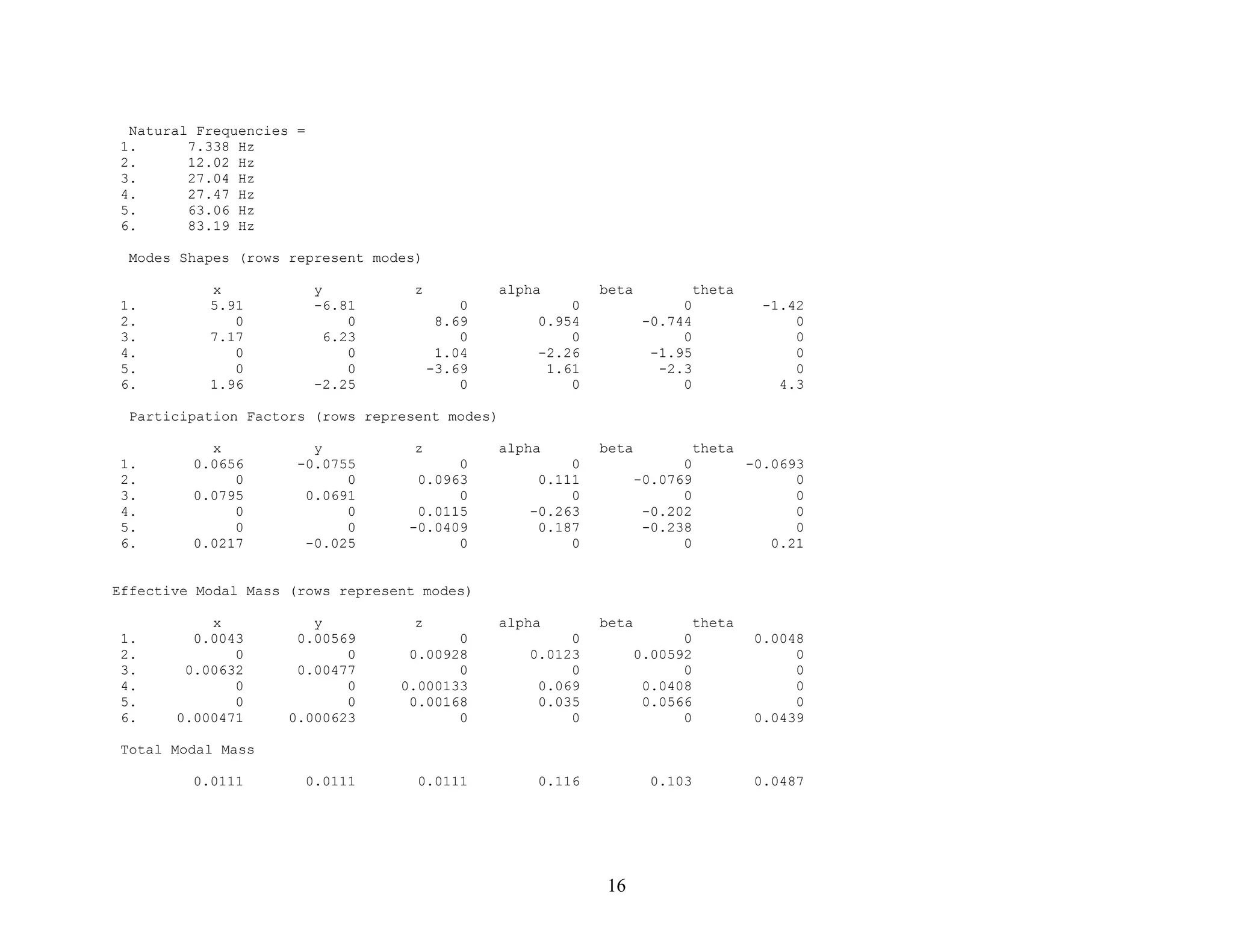
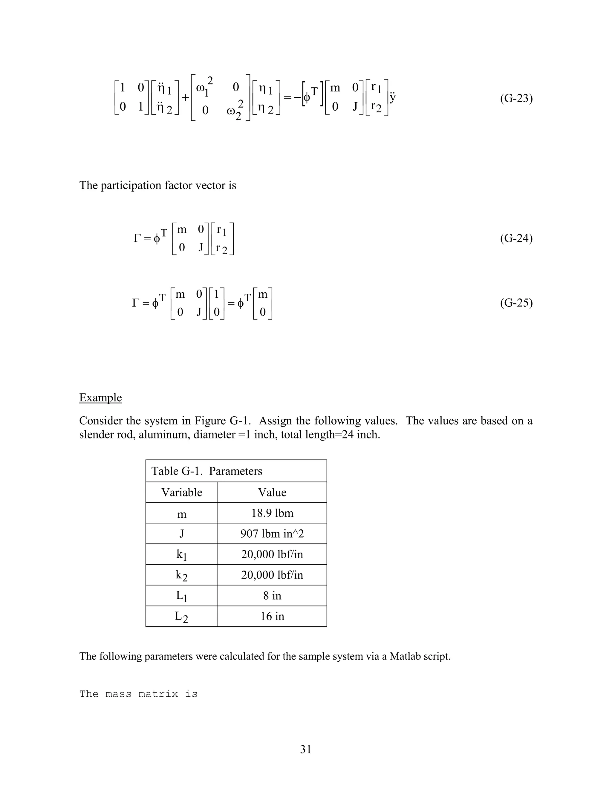
3) An example calculation is shown for a two degree-of-freedom system to demonstrate how to compute its eigenvalues, eigenvectors, and then the effective modal masses and participation factors of each mode. The first mode is found to have much higher effective mass


![Stress_and_Strain_Analysis[1].pptx](https://cdn.slidesharecdn.com/ss_thumbnails/stressandstrainanalysis1-230629101214-bc6c0ced-thumbnail.jpg?width=640&height=640&fit=bounds)