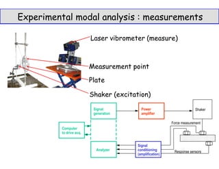
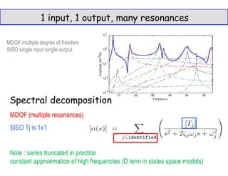
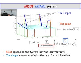
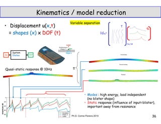
1. The document discusses experimental modal analysis which involves exciting a structure using a shaker, measuring the response using a laser vibrometer, and analyzing the transfer functions between the input and output using a computer. 2. It describes how modal analysis can be used to model a structure as a multiple-degree-of-freedom system with multiple resonances, and how the modes can be estimated from time signals. 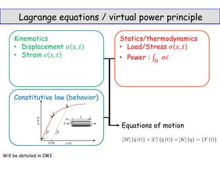3. Lagrange equations are mentioned as a way to derive the equations of motion for a structure based on its kinetic energy, strain energy, and work done by external loads.

1. Shaker (excitation)
Plate
Laser vibrometer (measure)
Measurement point
Experimental modal analysis : measurements
Computer
to drive acq.
Signal
generation
Power
amplifier
Shaker
Force measurement
Response sensors
Signal
conditioning
(amplification)
Analyzer

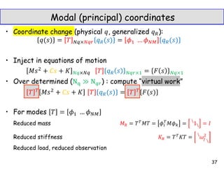
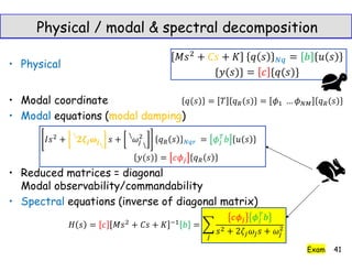
2. Bode plot : visualization of transfer function
Modal analysis : transfers
In
U
Out
Y
System H
{Y(w)}=[H(w)]{U(w)}
ONE input
ONE output
MANY resonances
Transfers estimated
from time response

3. 1 input, 1 output, many resonances
Spectral decomposition
MDOF (multiple resonances)
SISO Tj is 1x1
Note : series truncated in practice
constant approximation of high frequencies (D term in states space models)
MDOF multiple degree of freedom
SISO single input single output

4. MDOF MIMO system
• Poles depend on the system (not the input/output)
• The shape is associated with the input/output locations
The shapes
The poles

5. Lagrange equations / virtual power principle
Kinematics
• Displacement
• Strain
Statics/thermodynamics
• Load/Stress
• Power :
Constitutive law (behavior)
Equations of motion
Will be detailed in CM3

6. Kinetic energy (mass matrix)
Strain energy (stiffness matrix)
Work of external load (here constant)
Lagrangian
Lagrange equations of motion (generally valid for NL non-linear systems)
Leads to
Lagrange equations (in advance of CM3 needed TD2)

7. Modes : harmonic solution with no force
complex mode (general definition)
Eigenvalue problem
Linear time invariant
https://www.youtube.com/watch?v=zstmGnaaaCI

8. • Real mode : no damping / elastic / conservative
• M>0 & K0  f real
• There are distinct modes for DOF
• Full solver : scipy.linalg.eig (LAPACK Linear Algebra)
• Partial solvers exist, a few keywords
– scipy.sparse.linalg.eigs (Matlab eigs) : Arnoldi
– FEM Solvers : Lanczos (Krylov+conjugate gradient), AMLS
Normal modes of elastic structure
34

9. Normal modes of elastic structure
• Orthogonality
• Scaling conditions
• Unit mass
• Unit amplitude
35

10. Kinematics / model reduction
• Displacement u(x,t)
= shapes (x) x DOF (t) {q}N=
qR
Nx NR
T
Ph.D. Corine Florens 2010
In Out
System
States
Quasi-static response @ 10Hz =
• Modes : high energy, load independent
(no blister shape)
• Static response (influence of input=blister),
important away from resonance
36
Variable separation

11. Modal (principal) coordinates
• Coordinate change (physical , generalized ):
• Inject in equations of motion
• Over determined ( ) : compute “virtual work”
• For modes
Reduced mass
Reduced stiffness
Reduced load, reduced observation
37

12. Observation
• {y} outputs are linearly related to DOFs {q} using an
observation equation
• Simple case : extraction
• More general : intermediate points, reactions,
strains, stresses, …
Illustrations TD1 (q3f, q6f) TD3 (q3a), TD5, …
38

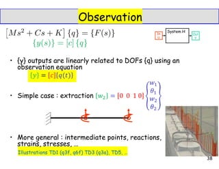
13. Command
• Loads decomposed as spatially unit loads and inputs
{F(t)} = [b] {u(t)}
Abaqus : *CLOAD + *AMPLITUDE, …
NASTRAN : FORCE-MOMENT + RLOAD
ANSYS, CODE Aster, …
Illustrations TD1, 3, 5, …
39

14. Rayleigh damping
– Physical domain
– Modal domain
= 𝒋 𝒋
Modal damping derived from test
40
Modal damping
O. Vo Van, E. Balmes, et X. Lorang, « Damping characterization of a high speed train catenary »,
IAVSD, Graz, 2015, http://sam.ensam.eu/handle/10985/10918.
Reality
Mass
Stiffness
can be > 100%
Physical domain 𝒋 𝒋

15. • Physical
• Modal coordinate
• Modal equations (modal damping)
𝒋 𝒋
• Reduced matrices = diagonal
Modal observability/commandability
• Spectral equations (inverse of diagonal matrix)
41
Physical / modal & spectral decomposition
Exam

16. Observability/controllability
42

17. Mots clefs du CM
• Définition mathématique des modes pour un modèle discret,
orthogonalité, normalisation (s3.2)
• Expression de la fonction de transfert en base modale,
masse et raideur modale, expression des contributions sous
forme de série (formule (3.29))
• Observabilité f(3.4) et commandabilité f(3.3) modale f(3.35)
• Amortissement modal, amortissement de Rayleigh (s3.4)
• Troncature
43