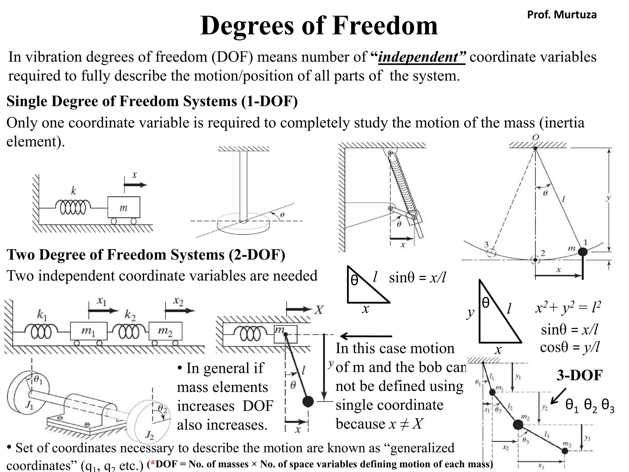
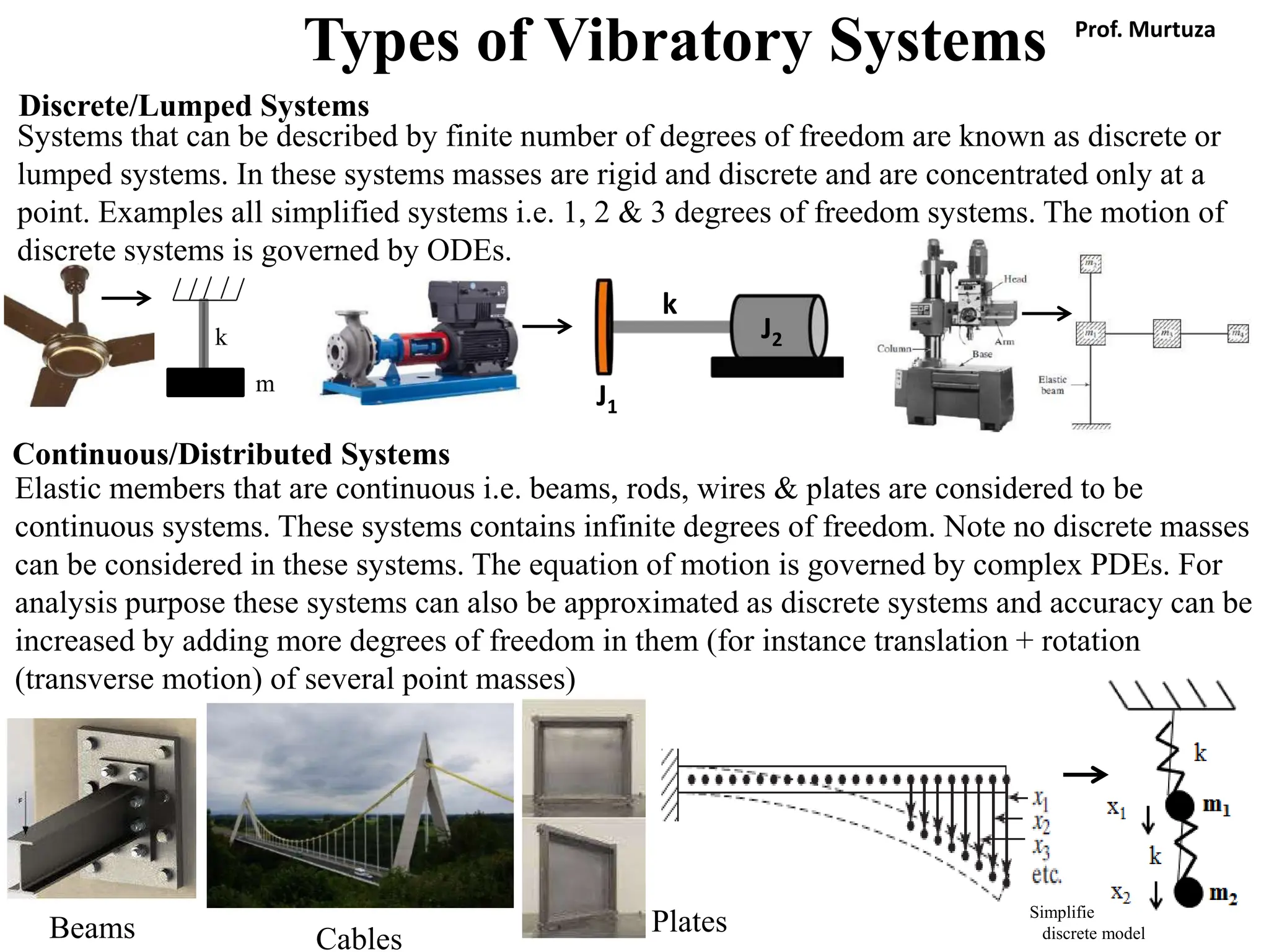
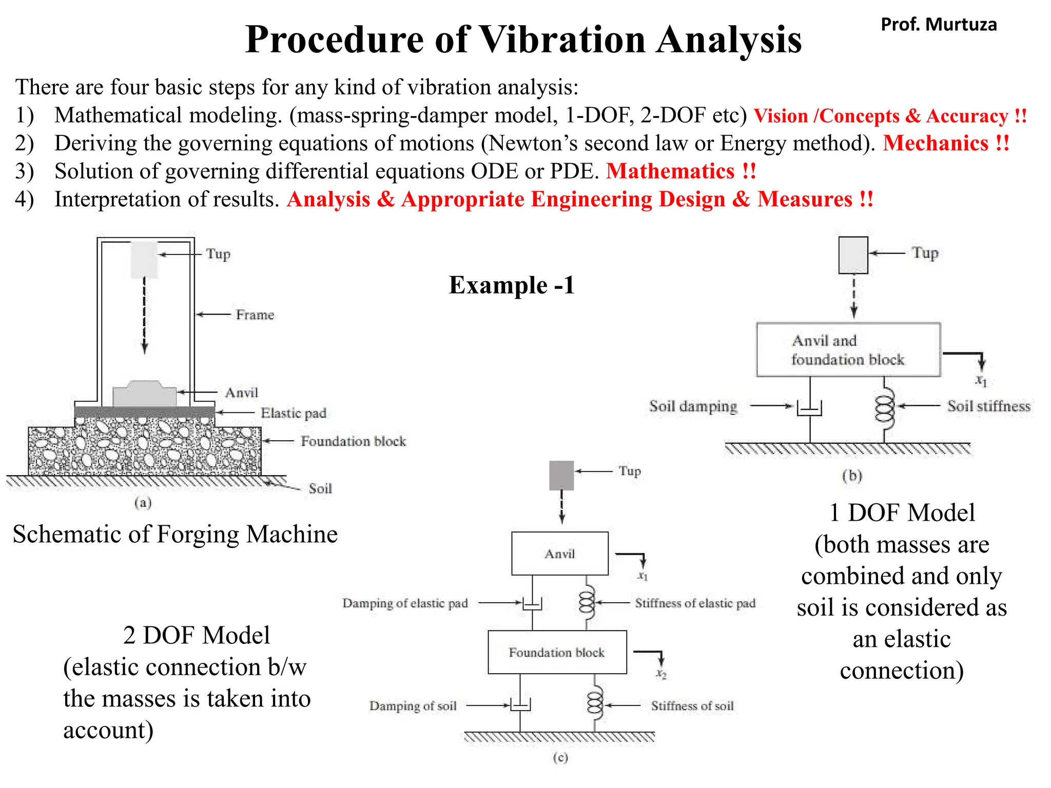
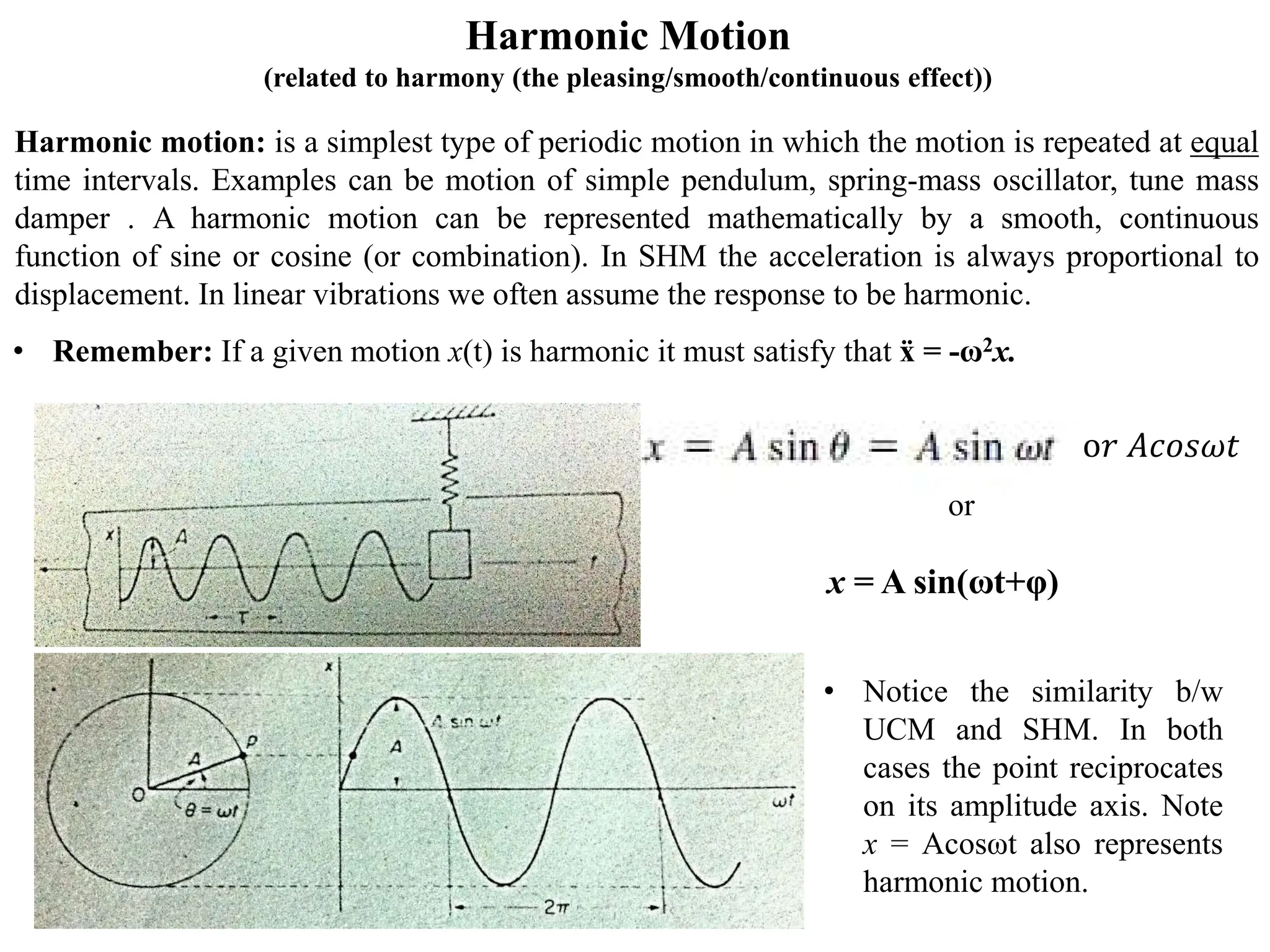
The document outlines the learning outcomes and course objectives for a mechanical vibrations class, emphasizing the theoretical and mathematical understanding of vibratory systems. Key concepts include mass, stiffness, natural frequency, degrees of freedom, and the classification of vibrations such as free and forced vibrations. It also addresses practical applications and the implications of vibrations in various mechanical systems, as well as the methods for vibration analysis.


![Decibel (dB)
• Unit for measuring the intensity of sound pressure level or simply sound level.
• It is the logarithmic ratio of vibration quantities like displacement, velocity, acceleration and
pressure. It measures the relative increase or decrease in a vibration quantity respect to some
reference. [+ve dB→ measured value is high & -ve dB→ measured value is less]
• Can be used in areas like acoustics, optics, electronics, digital imaging and video.
XdB = 20Log
𝑋𝑋
𝑋𝑋𝑜𝑜
X = measured quantity
Xo = reference value
Sound Proof Construction:
• Double glazed glass windows
with vacuum.
• Wall mounted acoustic panels
(mostly fiber glass but foam
rubber & animal furs &
feathers are also used)
• In general thicker and denser
material provide better sound
proofing but can be costly.
• Ratio of loudest sound
to weakest sound heard
by humans = 1 trillion
!!!](https://image.slidesharecdn.com/mv-250110055634-7096d62a/75/Fundamentals-of-Mechanical-Engineering-Vibrations-pdf-24-2048.jpg)

![Equivalent Damping
In order to estimate the equivalent damping of the system, same rules are applied as for
equivalent springs.
Viscous Damping:
The most commonly used damping method e.g. pneumatic and hydraulic piston cylinder dashpot.
The resistance is provided by the viscosity of a fluid (gas or oil). Damping force is not a constant.
NOTE:
Damping force Fd = -c ẋ= - cv This force is opposite (-ve) to the motion of the body
& will only exist if there is some relative velocity between the two ends of a damper.
Coulomb Damping:
This damping takes place when two solid materials rub against each other. The damping force remains
constant. It is due to dry friction. Example piston motion inside a cylinder block with low lubrication.
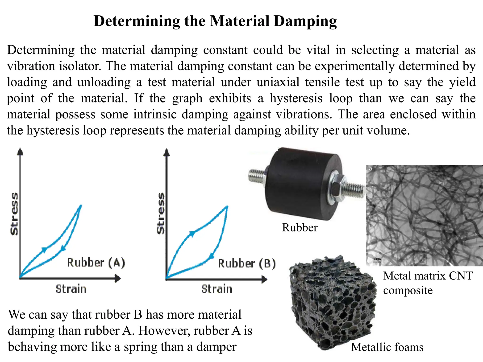
Material Damping:
This damping takes place when atomic planes within the material slide/slip relative to each other
when the material is deformed. It is due to friction between the atomic planes. Rubber has high
material damping.
c = Damping constant [Ns/m]
ct = [Nsm] in torsion!
𝑐𝑐𝑒𝑒𝑒𝑒 = 4𝜇𝜇𝜇𝜇𝜇𝜇
𝜋𝜋𝜋𝜋𝑥𝑥
�
𝑐𝑐𝑒𝑒𝑒𝑒 = ℎ
𝜔𝜔
� h = material damping constant
μ = static friction coefficient
ω = frequency [rad/s]](https://image.slidesharecdn.com/mv-250110055634-7096d62a/75/Fundamentals-of-Mechanical-Engineering-Vibrations-pdf-27-2048.jpg)


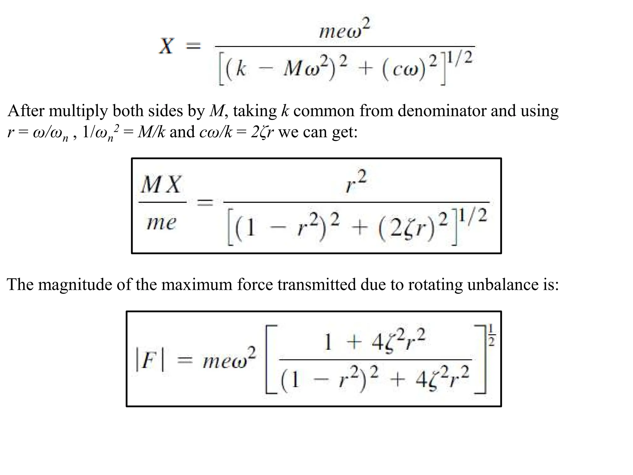


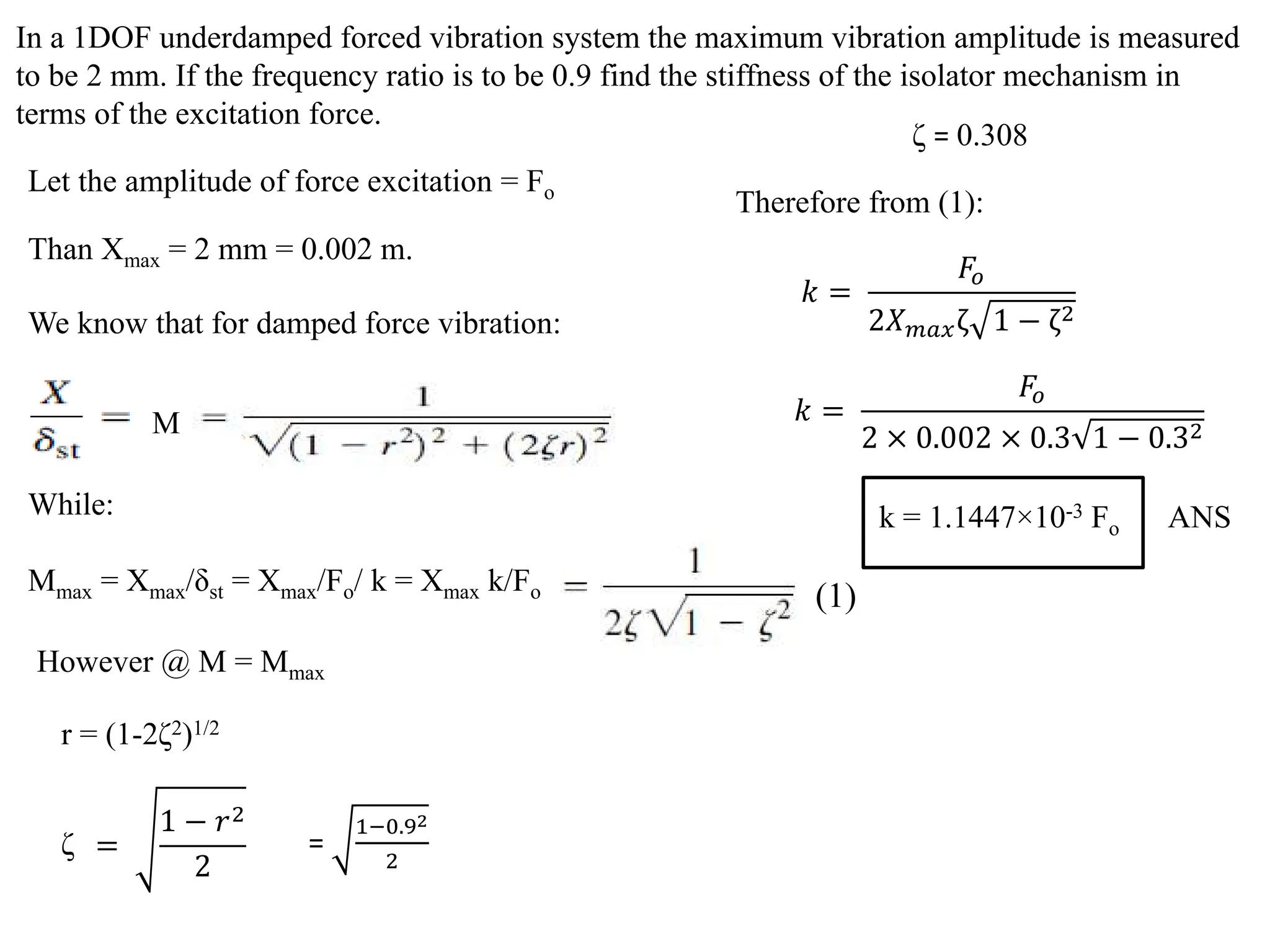
![Taking k as common and using following substitutions we can write:
ωn = (k/m)1/2 , c = 2ζmωn , δst = Fo/k , r = ω/ωn , X/δst = M (magnification factor)
[(1-mω2/k)2 + c2ω2/k2]1/2
/k
= = M
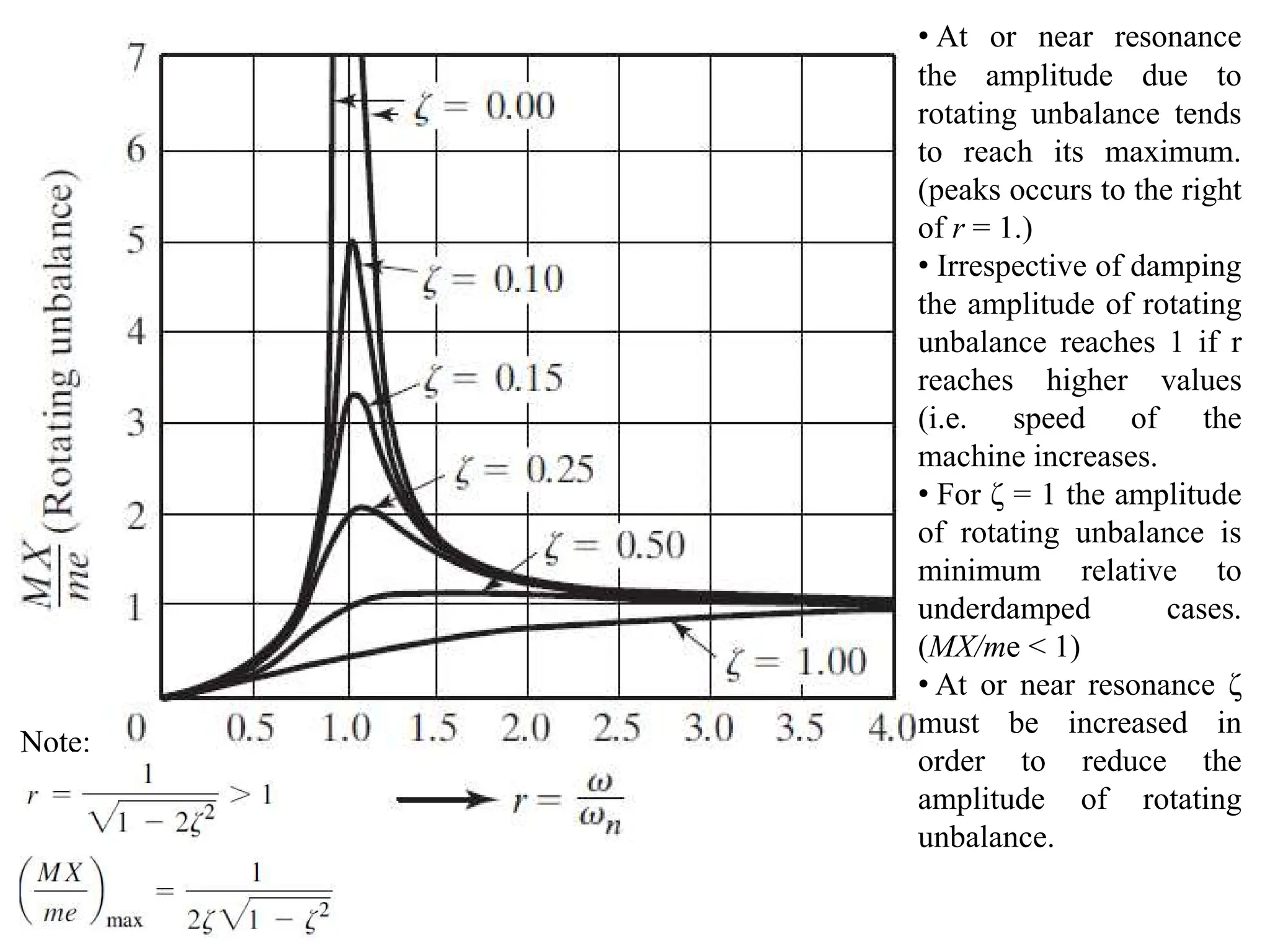
As before, the variation of magnification factor M with the frequency ratio r is
important for damped forced vibrations:
Therefore,
Therefore, for damped forced vibrations we have:
M
Note:
From dM/dr =0 we get
Mmax @ r = (1-2ζ2)1/2
Prof. Dr. Murtuza (NEDUET)](https://image.slidesharecdn.com/mv-250110055634-7096d62a/75/Fundamentals-of-Mechanical-Engineering-Vibrations-pdf-91-2048.jpg)