Download as PDF, PPTX


![Hierarchical
representations
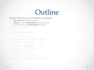
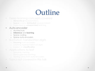
“Deep learning methods aim at
learning feature hierarchies
with features from higher levels
of the hierarchy formed by the
composition of lower level
features.
Automatically learning features
at multiple levels of abstraction
allows a system
to learn complex functions
mapping the input to the output
directly from data,
without depending completely
on human-crafted features.”
— Yoshua Bengio
[Bengio, “On the expressive power of deep architectures”, Talk at ALT, 2011]
[Bengio, Learning Deep Architectures for AI, 2009]](https://image.slidesharecdn.com/autoencoders-181001033311/85/Introduction-to-Autoencoders-6-320.jpg)
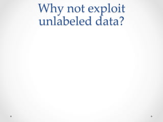
![Sparse and/or distributed
representations
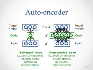
Example on MNIST handwritten digits
An image of size 28x28 pixels can be represented
using a small combination of codes from a basis set.
+ 1 + 1= 1 + 1 + 1 + 1 + 1 + 0.8 + 0.8
Figure 4: Top: A randomly selected subset of encoder filters learned by our energy-based model
when trained on the MNIST handwritten digit dataset. Bottom: An example of reconstruction of a
digit randomly extracted from the test data set. The reconstruction is made by adding “parts”: it is
the additive linear combination of few basis functions of the decoder with positive coefficients.
Examples of learned encoder and decoder filters are shown in figure 3. They are spatially localized,
and have different orientations, frequencies and scales. They are somewhat similar to, but more
localized than, Gabor wavelets and are reminiscent of the receptive fields of V1 neurons. Interest-
ingly, the encoder and decoder filter values are nearly identical up to a scale factor. After training,
inference is extremely fast, requiring only a simple matrix-vector multiplication.
[Ranzato, Poultney, Chopra & LeCun, “Efficient Learning of Sparse Representations with an Energy-‐‑Based Model ”, NIPS, 2006;
Ranzato, Boureau & LeCun, “Sparse Feature Learning for Deep Belief Networks ”, NIPS, 2007]
Biological motivation: V1 visual cortex](https://image.slidesharecdn.com/autoencoders-181001033311/85/Introduction-to-Autoencoders-7-320.jpg)
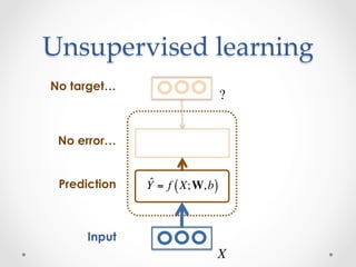
![Sparse and/or distributed
representations
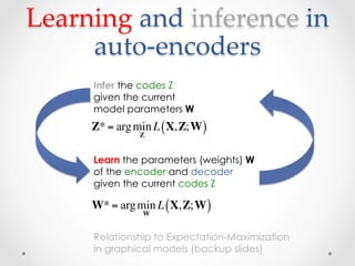
Example on MNIST handwritten digits
An image of size 28x28 pixels can be represented
using a small combination of codes from a basis set.
+ 1 + 1= 1 + 1 + 1 + 1 + 1 + 0.8 + 0.8
Figure 4: Top: A randomly selected subset of encoder filters learned by our energy-based model
when trained on the MNIST handwritten digit dataset. Bottom: An example of reconstruction of a
digit randomly extracted from the test data set. The reconstruction is made by adding “parts”: it is
the additive linear combination of few basis functions of the decoder with positive coefficients.
Examples of learned encoder and decoder filters are shown in figure 3. They are spatially localized,
and have different orientations, frequencies and scales. They are somewhat similar to, but more
localized than, Gabor wavelets and are reminiscent of the receptive fields of V1 neurons. Interest-
ingly, the encoder and decoder filter values are nearly identical up to a scale factor. After training,
inference is extremely fast, requiring only a simple matrix-vector multiplication.
At the end of this talk, you should know how to learn that basis set
and how to infer the codes, in a 2-layer auto-encoder architecture.
Matlab/Octave code and the MNIST dataset will be provided.
[Ranzato, Poultney, Chopra & LeCun, “Efficient Learning of Sparse Representations with an Energy-‐‑Based Model ”, NIPS, 2006;
Ranzato, Boureau & LeCun, “Sparse Feature Learning for Deep Belief Networks ”, NIPS, 2007]
Biological motivation: V1 visual cortex (backup slides)](https://image.slidesharecdn.com/autoencoders-181001033311/85/Introduction-to-Autoencoders-8-320.jpg)


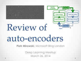
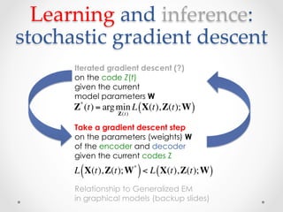
![Examples of
unsupervised learning
• Linear decomposition of the inputs:
o Principal Component Analysis and Singular Value Decomposition
o Independent Component Analysis [Bell & Sejnowski, 1995]
o Sparse coding [Olshausen & Field, 1997]
o …
• Fitting a distribution to the inputs:
o Mixtures of Gaussians
o Use of Expectation-Maximization algorithm [Dempster et al, 1977]
o …
• For text or discrete data:
o Latent Semantic Indexing [Deerwester et al, 1990]
o Probabilistic Latent Semantic Indexing [Hofmann et al, 1999]
o Latent Dirichlet Allocation [Blei et al, 2003]
o Semantic Hashing
o …](https://image.slidesharecdn.com/autoencoders-181001033311/85/Introduction-to-Autoencoders-15-320.jpg)


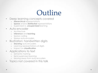
![Stacking auto-‐‑encoders
Code
Input
Code prediction
Code energy
Decoding energy
Input decoding
Sparsity
constraint
X
Z
Code
Input
Code prediction
Code energy
Decoding energy
Input decoding
Sparsity
constraint
X
Z
[Ranzato, Boureau & LeCun, “Sparse Feature Learning for Deep Belief Networks ”, NIPS, 2007]
Video:
Autoencoder applications:
https://www.youtube.com/watch?
v=J4DsymeZe2g](https://image.slidesharecdn.com/autoencoders-181001033311/85/Introduction-to-Autoencoders-29-320.jpg)
![MNIST handwricen digits
• Database of 70k
handwritten digits
o Training set: 60k
o Test set: 10k
• 28 x 28 pixels
• Best performing
classifiers:
o Linear classifier: 12% error
o Gaussian SVM 1.4% error
o ConvNets <1% error
[hcp://yann.lecun.com/exdb/mnist/]
https://blog.keras.io/building-autoenc
oders-in-keras.html](https://image.slidesharecdn.com/autoencoders-181001033311/85/Introduction-to-Autoencoders-30-320.jpg)
![Stacked auto-‐‑encoders
Code
Input
Code prediction
Code energy
Decoding energy
Input decoding
Sparsity
constraint
X
Z
Code
Input
Code prediction
Code energy
Decoding energy
Input decoding
Sparsity
constraint
X
Z
(C)
0 0.5 1 1.5 2
0.05
0.1
0.15
Entropy (bits/pixel) (D)
(E) (F)
(G) (H)
Figure 1: (A)-(B) Error rate on MNIST training (with 10, 100 a
test set produced by a linear classifier trained on the codes produ
The entropy and RMSE refers to a quantization into 256 bins. The
also to the same classifier trained on raw pixel data (showing the a
The error bars refer to 1 std. dev. of the error rate for 10 rand
(same splits for all methods). The parameter αs in eq. 8 takes va
Comparison between SESM, RBM, and PCA when quantizing the
Random selection from the 200 linear filters that were learned by SE
of original and reconstructed digit from the code produced by the
propagation through encoder and decoder). (F) Random selection
Back-projection in image space of the filters learned in the second
extractor. The second stage was trained on the non linearly transfor
stage machine. The back-projection has been performed by using a
machine, and propagating this through the second stage decoder an
at the second stage discover the class-prototypes (manually order
though no class label was ever used during training. (H) Feature ex
patches: some filters that were learned.
(A)
0 1 2
0
5
10
15
20
25
30
35
40
45
ENTROPY (bits/pixel)
ERRORRATE%
10 samples
0 1 2
0
2
4
6
8
10
12
14
16
18
ENTROPY (bits/pixel)
ERRORRATE%
100 samples
0 1 2
3
4
5
6
7
8
9
10
ENTROPY (bits/pixel)
ERRORRATE%
1000 samples
RAW: train
RAW: test
PCA: train
PCA: test
RBM: train
RBM: test
SESM: train
SESM: test
(B)
0 0.2 0.4
0
5
10
15
20
25
30
35
40
45
RMSE
ERRORRATE%
10 samples
0 0.2 0.4
0
2
4
6
8
10
12
14
16
18
RMSE
ERRORRATE%
100 samples
0 0.2 0.4
3
4
5
6
7
8
9
10
RMSE
ERRORRATE%
1000 samples
(C)
0 0.5 1 1.5 2
0.05
0.1
0.15
0.2
0.25
0.3
0.35
0.4
0.45
RMSE
Entropy (bits/pixel)
Symmetric Sparse Coding − RBM − PCA
PCA: quantization in 5 bins
PCA: quantization in 256 bins
RBM: quantization in 5 bins
RBM: quantization in 256 bins
Sparse Coding: quantization in 5 bins
Sparse Coding: quantization in 256 bins
(D)
Layer 1: Matrix W1 of size 192 x 784
192 sparse bases of 28 x 28 pixels
Layer 2: Matrix W2 of size 10 x 192
10 sparse bases of 192 units
[Ranzato, Boureau & LeCun, “Sparse Feature Learning for Deep Belief Networks ”, NIPS, 2007]](https://image.slidesharecdn.com/autoencoders-181001033311/85/Introduction-to-Autoencoders-31-320.jpg)


![Semantic Hashing
[Hinton & Salakhutdinov, “Reducing the dimensionality of data with neural networks, Science, 2006;
Salakhutdinov & Hinton, “Semantic Hashing”, Int J Approx Reason, 2007]
2000
500
250
125
2
125
250
500
2000](https://image.slidesharecdn.com/autoencoders-181001033311/85/Introduction-to-Autoencoders-35-320.jpg)
![Beyond auto-‐‑encoders
for web search (MSR)
[Huang, He, Gao, Deng et al, “Learning Deep Structured Semantic Models for Web Search using Clickthrough Data”, CIKM, 2013]
s: “racing car”Input word/phrase
dim = 5MBag-of-words vector
dim = 50K
d=500Letter-tri-gram
embedding matrix
Letter-tri-gram coeff.
matrix (fixed)
d=500
Semantic
vector
d=300
t1: “formula one”
dim = 5M
dim = 50K
d=500
d=500
d=300
t2: “ford model t”
dim = 5M
dim = 50K
d=500
d=500
d=300
Compute Cosine similarity
between semantic vectors cos(s,t1) cos(s,t2)
W1
W2
W3
W4](https://image.slidesharecdn.com/autoencoders-181001033311/85/Introduction-to-Autoencoders-36-320.jpg)

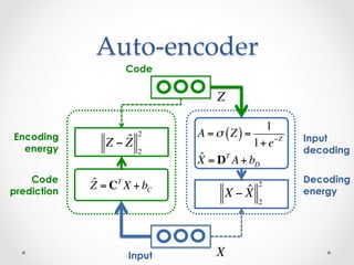
The document provides an introduction and overview of auto-encoders, including their architecture, learning and inference processes, and applications. It discusses how auto-encoders can learn hierarchical representations of data in an unsupervised manner by compressing the input into a code and then reconstructing the output from that code. Sparse auto-encoders and stacking multiple auto-encoders are also covered. The document uses handwritten digit recognition as an example application to illustrate these concepts.