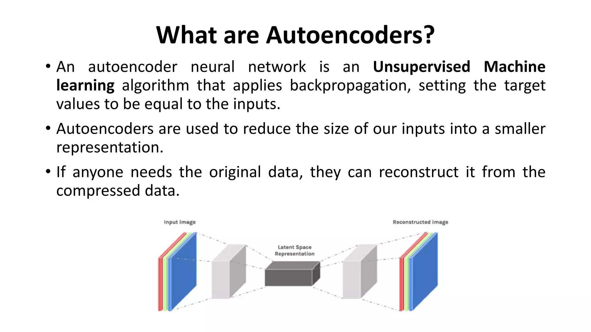
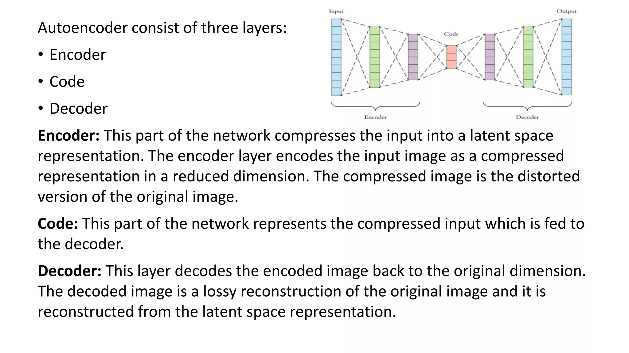
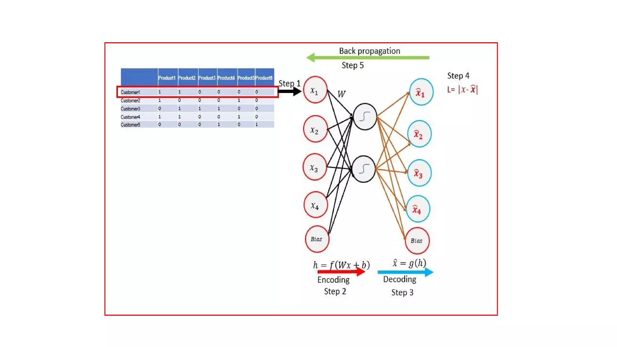
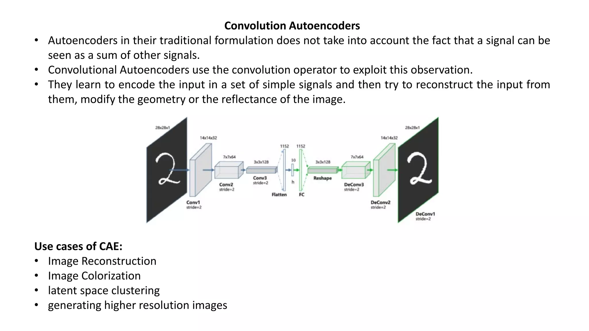
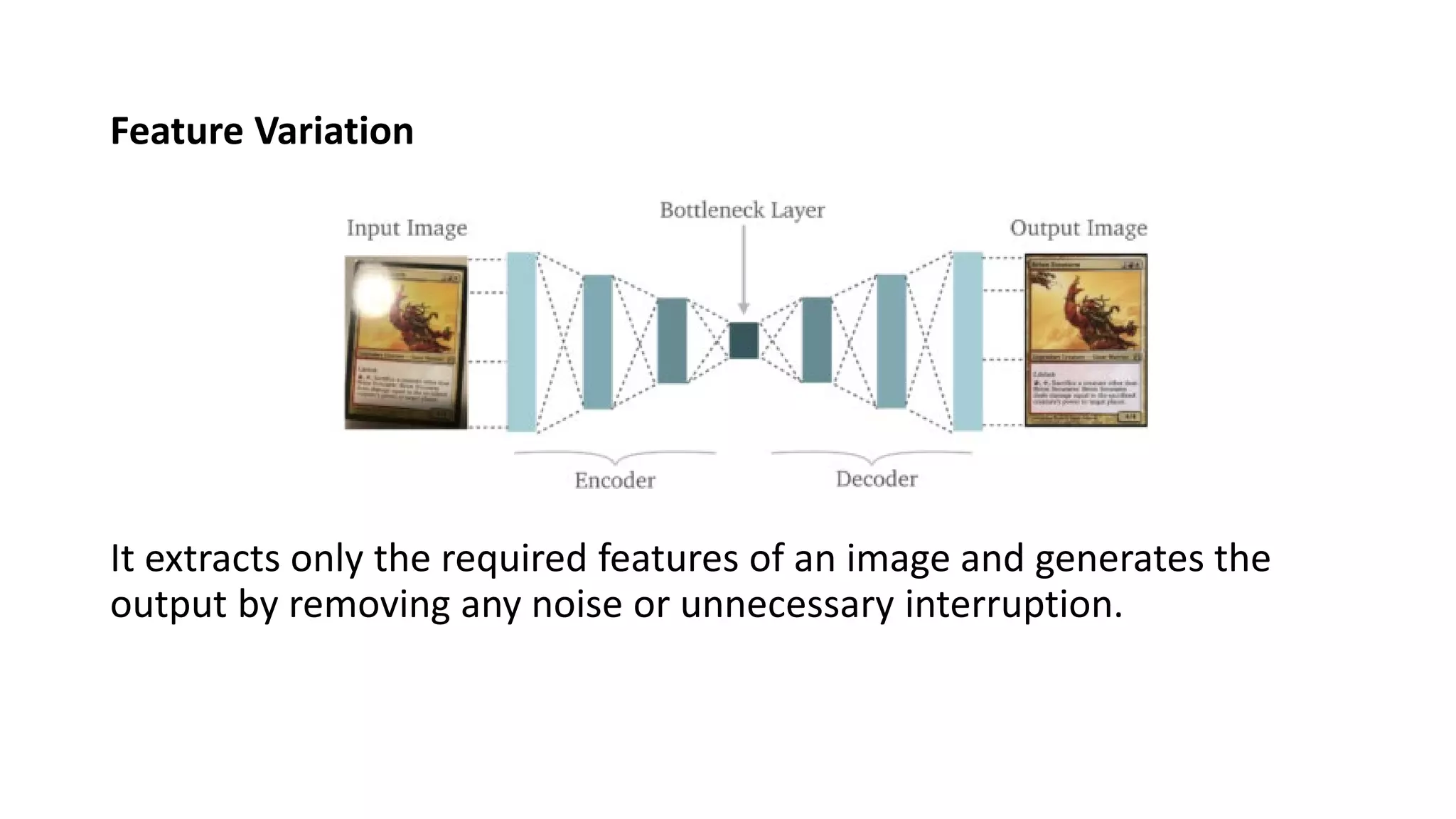
- Autoencoders are unsupervised neural networks that compress input data into a latent space representation and then reconstruct the output from this representation. They aim to copy their input to their output with minimal loss of information. - Autoencoders consist of an encoder that compresses the input into a latent space and a decoder that decompresses this latent space back into the original input space. The network is trained to minimize the reconstruction loss between the input and output. 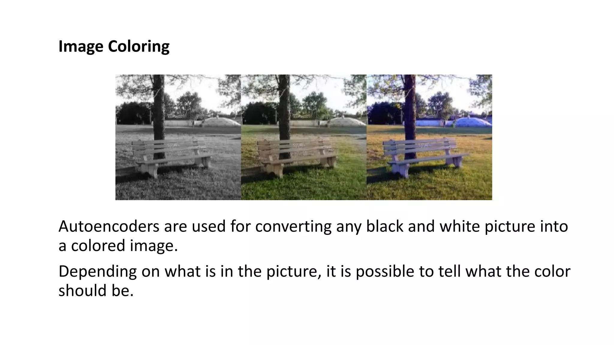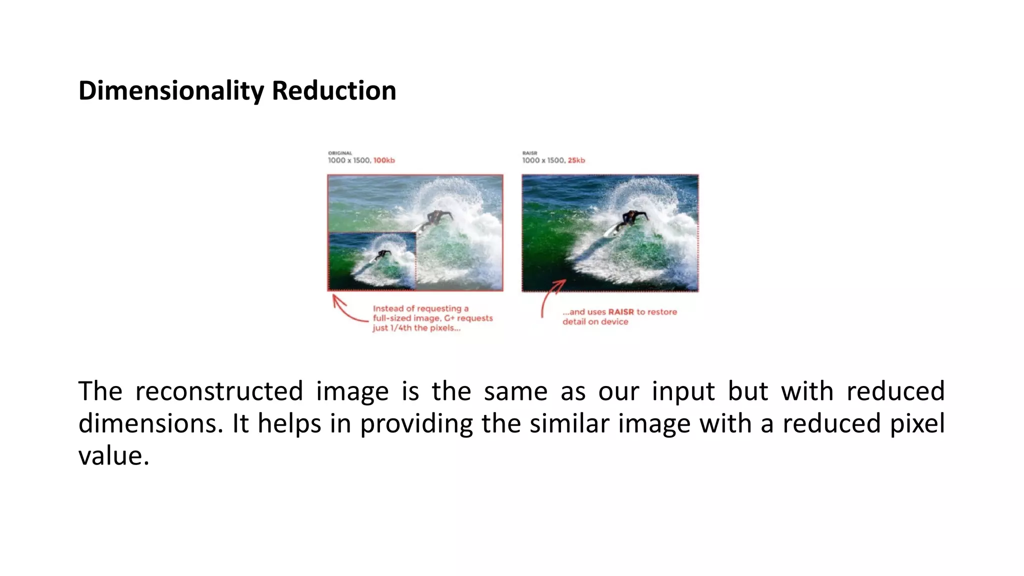- Autoencoders are commonly used for dimensionality reduction, feature extraction, denoising images, and generating new data similar to the training data distribution.

1. UNIT-4
Autoencoders

2. What are Autoencoders?
• An autoencoder neural network is an Unsupervised Machine
learning algorithm that applies backpropagation, setting the target
values to be equal to the inputs.
• Autoencoders are used to reduce the size of our inputs into a smaller
representation.
• If anyone needs the original data, they can reconstruct it from the
compressed data.

3. Autoencoder
• An autoencoder is an unsupervised machine learning algorithm that takes an image
as input and tries to reconstruct it using fewer number of bits from the bottleneck
also known as latent space.
• The image is majorly compressed at the bottleneck.
• The compression in autoencoders is achieved by training the network for a period of
time and as it learns it tries to best represent the input image at the bottleneck.
• The general image compression algorithms like JPEG and JPEG lossless
compression techniques compress the images without the need for any kind of
training and do fairly well in compressing the images.
• Autoencoders are similar to dimensionality reduction techniques like Principal
Component Analysis (PCA).
• They project the data from a higher dimension to a lower dimension using linear
transformation and try to preserve the important features of the data while
removing the non-essential parts.

4. • However, the major difference between autoencoders and PCA lies in the transformation
part: as you already read, PCA uses linear transformation whereas autoencoders use non-
linear transformations.
• Now that you have a bit of understanding about autoencoders, let's now break this term
and try to get some intuition about it!
• The above figure is a two-layer autoencoder with one hidden layer.
• In deep learning terminology, you will often notice that the input layer is never taken into
account while counting the total number of layers in an architecture.
• The total layers in an architecture only comprises of the number of hidden layers and the
output layer.

5. • As shown in the image above, the input and output layers have the same number
of neurons.
• Let's take an example. You feed an image with just five pixel values into the
autoencoder which is compressed by the encoder into three pixel values at the
bottleneck (middle layer) or latent space.
• Using these three values, the decoder tries to reconstruct the five pixel values or
rather the input image which you fed as an input to the network.

6. The need of Autoencoders
A similar machine learning algorithm ie. PCA which does the same task. But,
autoencoders are preferred over PCA because
• An autoencoder can learn non-linear transformations
with a non-linear activation function and multiple layers.
• It doesn’t have to learn dense layers. It can use
convolutional layers to learn which is better for video,
image and series data.
• It is more efficient to learn several layers with an
autoencoder rather than learn one huge transformation
with PCA.
• An autoencoder provides a representation of each layer
as the output.
• It can make use of pre-trained layers from another model
to apply transfer learning to enhance the
encoder/decoder.

7. Need of Autoencoders
• Used for Non Linear Dimensionality Reduction: Encodes input in the hidden layer
to a smaller dimension compared to the input dimension. Hidden layer is later
decoded as output. Output layer has the same dimension as input. Autoencoder
reduces dimensionality of linear and nonlinear data hence it is more powerful than
PCA.
• Used in Recommendation Engines: This uses deep encoders to understand user
preferences to recommend movies, books or items
• Used for Feature Extraction : Autoencoders tries to minimize the reconstruction error.
In the process to reduce the error, it learns some of important features present in the
input. It reconstructs the input from the encoded state present in the hidden layer.
Encoding generates a new set of features which is a combination of the original
features. Encoding in autoencoders helps to identify the latent features presents in the
input data.
• Image recognition : Stacked autoencoder are used for image recognition. We can use
multiple encoders stacked together helps to learn different features of an image.

8. Applications of
Autoencoders

9. Image Coloring
Autoencoders are used for converting any black and white picture into
a colored image.
Depending on what is in the picture, it is possible to tell what the color
should be.

10. Feature Variation
It extracts only the required features of an image and generates the
output by removing any noise or unnecessary interruption.

11. Dimensionality Reduction
The reconstructed image is the same as our input but with reduced
dimensions. It helps in providing the similar image with a reduced pixel
value.

13. Denoising Image
The input seen by the autoencoder is not the raw input but a
stochastically corrupted version. A denoising autoencoder is thus
trained to reconstruct the original input from the noisy version.

14. Noised image Denoised image

15. Watermark Removal
It is also used for removing watermarks from images or to remove any
object while filming a video or a movie.
Now that you have an idea of the different industrial applications of
Autoencoders, let’s continue our article and understand the complex
architecture of Autoencoders.

16. Architecture of
Autoencoders

17. Autoencoder consist of three layers:
• Encoder
• Code
• Decoder
Encoder: This part of the network compresses the input into a latent space
representation. The encoder layer encodes the input image as a compressed
representation in a reduced dimension. The compressed image is the distorted
version of the original image.
Code: This part of the network represents the compressed input which is fed to
the decoder.
Decoder: This layer decodes the encoded image back to the original dimension.
The decoded image is a lossy reconstruction of the original image and it is
reconstructed from the latent space representation.

18. The layer between the encoder and decoder, ie. the
code is also known as Bottleneck. This is a well-
designed approach to decide which aspects of
observed data are relevant information and what
aspects can be discarded. It does this by balancing two
criteria :
• The compactness of representation, measured as the
compressibility.
• It retains some behaviorally relevant variables from
the input.
Now that you have an idea of the architecture of an
Autoencoder. Let’s continue and understand the
different properties and the Hyperparameters involved
while training Autoencoders.

19. Autoencoder Components
• Autoencoders consists of 4 main parts:
– Encoder: In which the model learns how to reduce the input dimensions
and compress the input data into an encoded representation.
– Bottleneck: which is the layer that contains the compressed
representation of the input data. This is the lowest possible dimensions
of the input data.
– Decoder: In which the model learns how to reconstruct the data from the
encoded representation to be as close to the original input as possible.
– Reconstruction Loss: This is the method that measures how well the decoder is
performing and how close the output is to the original input.
• The training then involves using back propagation in order to minimize the network’s
reconstruction loss.

20. How does Autoencoders work?
• We take the input, encode it to identify latent feature representation. Decode the
latent feature representation to recreate the input.
• We calculate the loss by comparing the input and output.
• To reduce the reconstruction error we back propagate and update the weights.
• Weight is updated based on how much they are responsible for the error.
• In our example, we have taken the dataset for products bought by customers.
• Step 1: Take the first row from the customer data for all products bought in an array as
the input. 1 represent that the customer bought the product. 0 represents that the
customer did not buy the product.
• Step 2: Encode the input into another vector h. h is a lower dimension vector than the
input. We can use sigmoid activation function for h as the it ranges from 0 to 1. W is the
weight applied to the input and b is the bias term.
h=f(Wx+b)

22. • Step 3: Decode the vector h to recreate the input. Output will be of same dimension as the
input.
• Step 4 : Calculate the reconstruction error L. Reconstruction error is the difference between
the input and output vector. Our goal is to minimize the reconstruction error so that output is
similar to the input vector
Reconstruction error= input vector — output vector
• Step 5: Back propagate the error from output layer to the input layer to update the weights.
Weights are updated based on how much they were responsible for the error. Learning rate
decides by how much we update the weights.
• Step 6: Repeat step 1 through 5 for each of the observation in the dataset. Weights
are updated after each
• Step 7: Repeat more epochs. Epoch is when all the rows in the dataset has passed through the
neural network.

23. Properties and
Hyperparameters

24. Properties of Autoencoders:
• Data-specific: Autoencoders are only able to compress data similar to
what they have been trained on.
• Lossy: The decompressed outputs will be degraded compared to the
original inputs.
• Learned automatically from examples: It is easy to train specialized
instances of the algorithm that will perform well on a specific type of
input.

25. Hyperparameters of Autoencoders:
There are 4 hyperparameters that we need to set before training an
autoencoder:

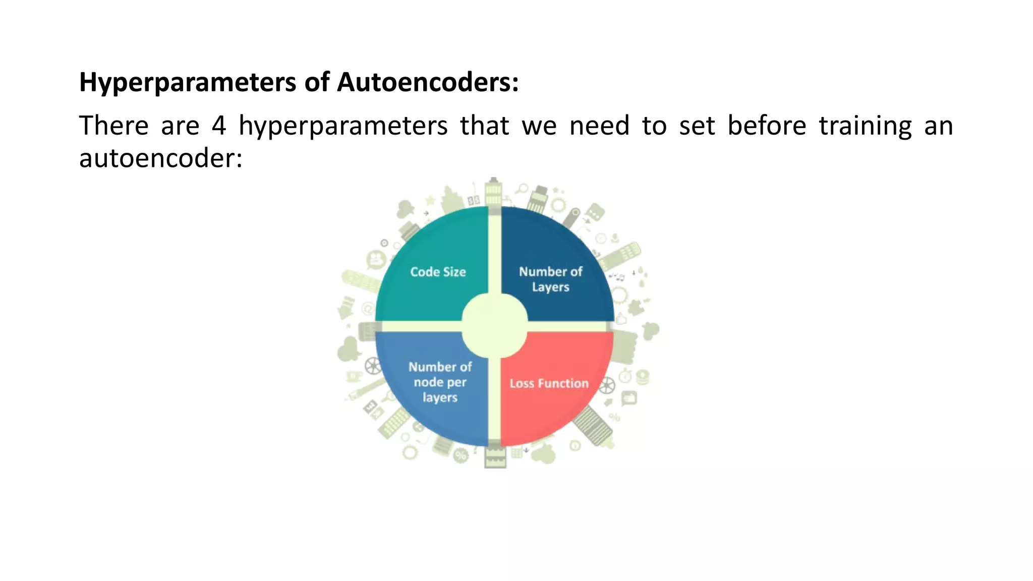
26. Code size: It represents the number of nodes in the middle layer.
Smaller size results in more compression.
Number of layers: The autoencoder can consist of as many layers as we
want.
Number of nodes per layer: The number of nodes per layer decreases
with each subsequent layer of the encoder, and increases back in the
decoder. The decoder is symmetric to the encoder in terms of the layer
structure.
Loss function: We either use mean squared error or binary cross-
entropy. If the input values are in the range [0, 1] then we typically use
cross-entropy, otherwise, we use the mean squared error.

27. 1. Simple Autoencoder
We begin by importing all the necessary libraries :
import all the dependencies
from keras.layers import Dense,Conv2D,MaxPooling2D,UpSampling2D
from keras import Input, Model
from keras.datasets import mnist
import numpy as np
import matplotlib.pyplot as plt
Then we will build our model and we will provide the number of dimensions that will decide how much the input
will be compressed. The lesser the dimension, the more will be the compression.
encoding_dim = 15
input_img = Input(shape=(784,))
# encoded representation of input
encoded = Dense(encoding_dim, activation='relu')(input_img)
# decoded representation of code
decoded = Dense(784, activation='sigmoid')(encoded)
# Model which take input image and shows decoded images
autoencoder = Model(input_img, decoded)
IMPLEMENTATION

28. Then we need to build the encoder model and decoder model separately so that we can easily differentiate
between the input and output.
# This model shows encoded images
encoder = Model(input_img, encoded)
# Creating a decoder model
encoded_input = Input(shape=(encoding_dim,))
# last layer of the autoencoder model
decoder_layer = autoencoder.layers[-1]
# decoder model
decoder = Model(encoded_input, decoder_layer(encoded_input))
Then we need to compile the model with the ADAM optimizer and cross-entropy loss function fitment.
autoencoder.compile(optimizer='adam', loss='binary_crossentropy')
Then you need to load the data :
(x_train, y_train), (x_test, y_test) = mnist.load_data()
x_train = x_train.astype('float32') / 255.
x_test = x_test.astype('float32') / 255.
x_train = x_train.reshape((len(x_train), np.prod(x_train.shape[1:])))
x_test = x_test.reshape((len(x_test), np.prod(x_test.shape[1:])))
print(x_train.shape)
print(x_test.shape)

29. If you want to see how the data is actually, you can use the following line of code :
plt.imshow(x_train[0].reshape(28,28))
Then you need to train your model :
autoencoder.fit(x_train, x_train,
epochs=15,
batch_size=256,
validation_data=(x_test, x_test))
After training, you need to provide the input and you can plot the results using the following code :
encoded_img = encoder.predict(x_test)
decoded_img = decoder.predict(encoded_img)
plt.figure(figsize=(20, 4))
for i in range(5):
# Display original
ax = plt.subplot(2, 5, i + 1)
plt.imshow(x_test[i].reshape(28, 28))
plt.gray()
ax.get_xaxis().set_visible(False)
ax.get_yaxis().set_visible(False)
# Display reconstruction
ax = plt.subplot(2, 5, i + 1 + 5)
plt.imshow(decoded_img[i].reshape(28, 28))
plt.gray()
ax.get_xaxis().set_visible(False)
ax.get_yaxis().set_visible(False)
plt.show()

30. Types of
Autoencoders

31. Undercomplete Autoencoders
– Goal of the Autoencoder is to capture the most
important features present in the data.
– Undercomplete autoencoders have a smaller dimension
for hidden layer compared to the input layer. This helps to
obtain important features from the data.
– Objective is to minimize the loss function by penalizing
the g(f(x)) for being different from the input x.
– When decoder is linear and we use a mean squared
error loss function then undercomplete autoencoder
generates a reduced feature space similar to PCA.
– We get a powerful nonlinear generalization of PCA
when encoder function f and decoder function g are
non linear.
– Undercomplete autoencoders do not need any
regularization as they maximize the probability of data
rather than copying the input to the output.

32. Convolution Autoencoders
• Autoencoders in their traditional formulation does not take into account the fact that a signal can be
seen as a sum of other signals.
• Convolutional Autoencoders use the convolution operator to exploit this observation.
• They learn to encode the input in a set of simple signals and then try to reconstruct the input from
them, modify the geometry or the reflectance of the image.
Use cases of CAE:
• Image Reconstruction
• Image Colorization
• latent space clustering
• generating higher resolution images

33. Sparse Autoencoders
– Sparse autoencoders have hidden nodes greater than input
nodes. They can still discover important features from the data.
– Sparsity constraint is introduced on the hidden layer. This is to
prevent output layer copy input data.
– Sparse autoencoders have a sparsity penalty, Ω(h), a value close
to zero but not zero. Sparsity penalty is applied on the hidden
layer in addition to the reconstruction error. This prevents
overfitting.
– Sparse autoencoders take the highest activation values in the
hidden layer and zero out the rest of the hidden nodes. This
prevents autoencoders to use all of the hidden nodes at a time
and forcing only a reduced number of hidden nodes to be used.
– As we activate and inactivate hidden nodes for each row in the
dataset. Each hidden node extracts a feature from the data

34. Denoising Autoencoders(DAE)
– Denoising refers to intentionally adding noise to the raw input before providing
it to the network. Denoising can be achieved using stochastic mapping.
– Denoising autoencoders create a corrupted copy of the input by introducing
some noise. This helps to avoid the autoencoders to copy the input to the
output without learning features about the data.
– Corruption of the input can be done randomly by making some of the input as
zero. Remaining nodes copy the input to the noised input.
– Denoising autoencoders must remove the corruption to generate an output
that is similar to the input. Output is compared with input and not with
noised input. To minimize the loss function we continue until convergence
– Denoising autoencoders minimizes the loss function between the output node
and the corrupted input.
– Denoising helps the autoencoders to learn the latent representation present
in the data. Denoising autoencoders ensures a good representation is one that
can be derived robustly from a corrupted input and that will be useful for
recovering the corresponding clean input.
– Denoising is a stochastic autoencoder as we use a stochastic corruption
process to set some of the inputs to zero.

35. Stacked Denoising Autoencoders
• Stacked Autoencoders is a neural network with multiple layers of sparse
autoencoders
• When we add more hidden layers than just one hidden layer to an
autoencoder, it helps to reduce a high dimensional data to a smaller code
representing important features
• Each hidden layer is a more compact representation than the last hidden layer
• We can also denoise the input and then pass the data through the stacked
autoencoders called as stacked denoising autoencoders
• In Stacked Denoising Autoencoders, input corruption is used only for initial
denoising. This helps learn important features present in the data. Once the
mapping function f(θ) has been learnt. For further layers we use
uncorrupted input from the previous layers.
• After training a stack of encoders as explained above, we can use the output
of the stacked denoising autoencoders as an input to a stand alone
supervised machine learning like support vector machines or multi class
logistics regression.

36. Deep Autoencoders
• The extension of the simple Autoencoder is the Deep Autoencoder.
• The first layer of the Deep Autoencoder is used for first-order features in the raw input.
• The second layer is used for second-order features corresponding to patterns in the
appearance of first-order features.
• Deeper layers of the Deep Autoencoder tend to learn even higher-order features.
A deep autoencoder is composed of two, symmetrical deep-belief networks-
• First four or five shallow layers representing the encoding half of the net.
• The second set of four or five layers that make up the decoding half.
Use cases of Deep Autoencoders
• Image Search
• Data Compression
• Topic Modeling & Information Retrieval (IR)

37. 2. Deep CNN Autoencoder :
Since the input here is images, it does make more sense to use a Convolutional Neural network or CNN.
The encoder will be made up of a stack of Conv2D and max-pooling layer and the decoder will have a
stack of Conv2D and Upsampling Layer.
Code :
model = Sequential()
# encoder network
model.add(Conv2D(30, 3, activation= 'relu', padding='same', input_shape = (28,28,1)))
model.add(MaxPooling2D(2, padding= 'same'))
model.add(Conv2D(15, 3, activation= 'relu', padding='same'))
model.add(MaxPooling2D(2, padding= 'same'))
#decoder network
model.add(Conv2D(15, 3, activation= 'relu', padding='same'))
model.add(UpSampling2D(2))
model.add(Conv2D(30, 3, activation= 'relu', padding='same'))
model.add(UpSampling2D(2))
model.add(Conv2D(1,3,activation='sigmoid', padding= 'same')) # output layer
model.compile(optimizer= 'adam', loss = 'binary_crossentropy')
model.summary()
IMPLEMENTATION

38. Now you need to load the data and training the
model
(x_train, _), (x_test, _) = mnist.load_data()
x_train = x_train.astype('float32') / 255.
x_test = x_test.astype('float32') / 255.
x_train = np.reshape(x_train, (len(x_train), 28, 28,
1))
x_test = np.reshape(x_test, (len(x_test), 28, 28, 1))
model.fit(x_train, x_train,
epochs=15,
batch_size=128,
validation_data=(x_test, x_test))
Now you need to provide the input and plot the output for the
following results
pred = model.predict(x_test)
plt.figure(figsize=(20, 4))
for i in range(5):
# Display original
ax = plt.subplot(2, 5, i + 1)
plt.imshow(x_test[i].reshape(28, 28))
plt.gray()
ax.get_xaxis().set_visible(False)
ax.get_yaxis().set_visible(False)
# Display reconstruction
ax = plt.subplot(2, 5, i + 1 + 5)
plt.imshow(pred[i].reshape(28, 28))
plt.gray()
ax.get_xaxis().set_visible(False)
ax.get_yaxis().set_visible(False)
plt.show()

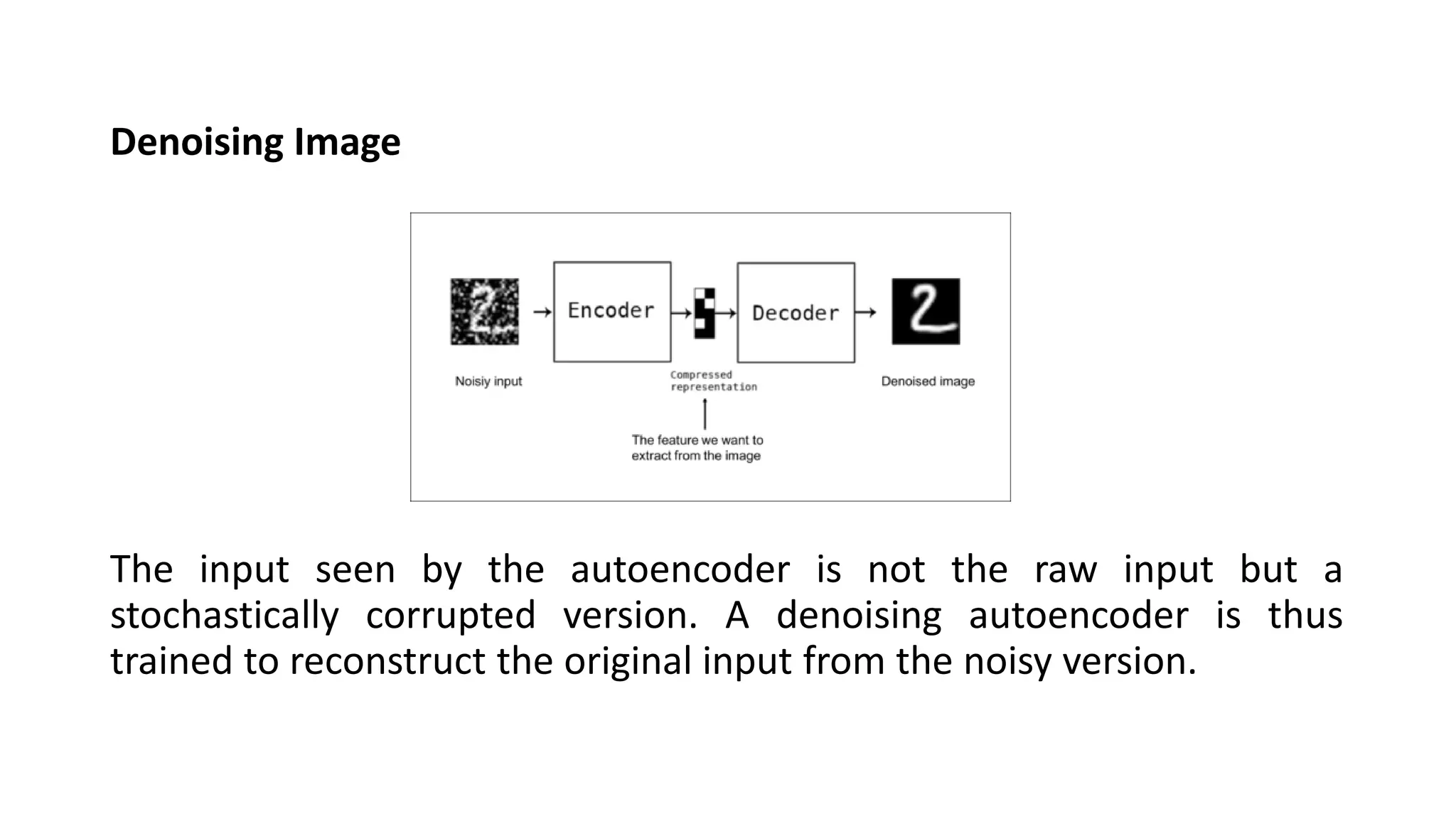
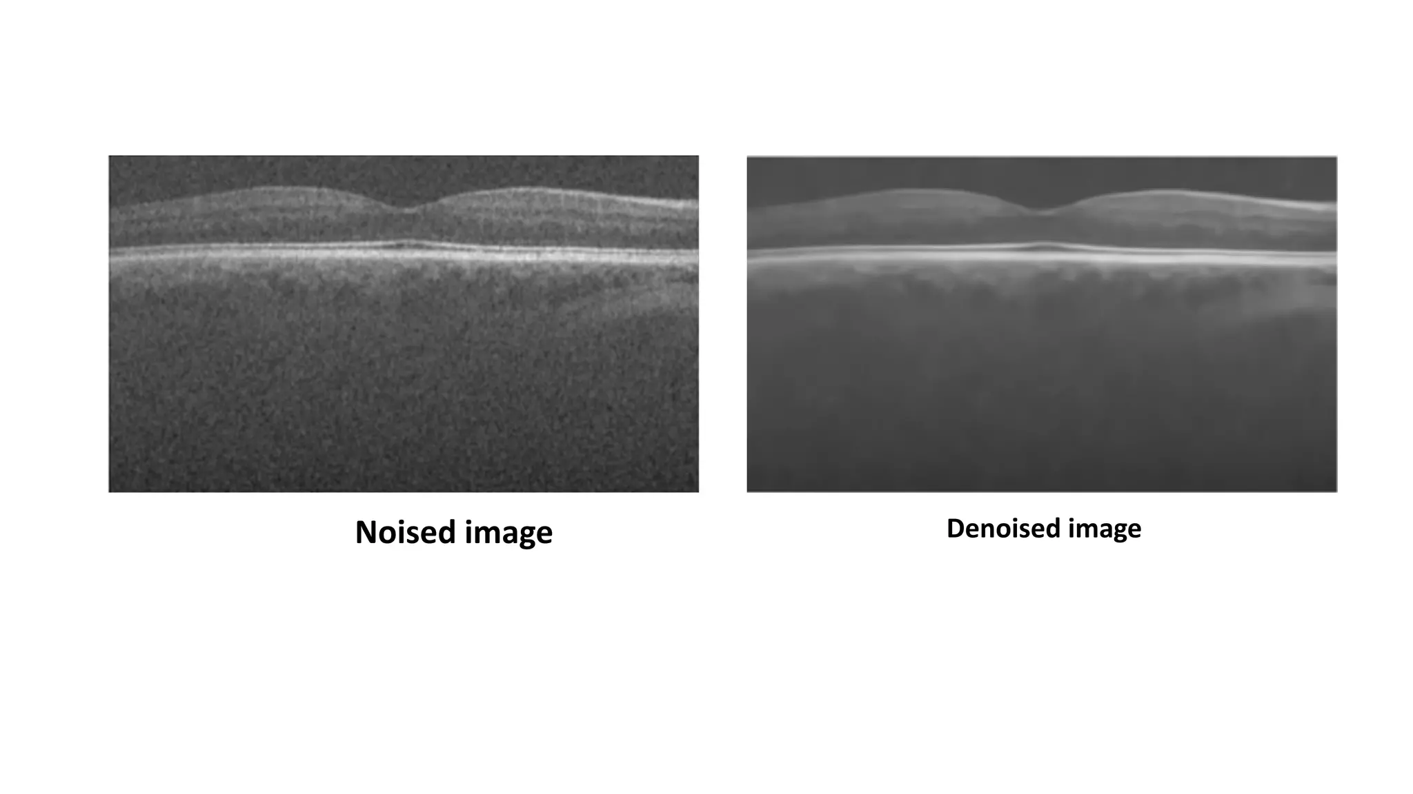
39. 3. Denoising Autoencoder
Now we will see how the model performs with noise in the image. What we mean by noise is blurry
images, changing the color of the images, or even white markers on the image.
noise_factor = 0.7
x_train_noisy = x_train + noise_factor * np.random.normal(loc=0.0, scale=1.0, size=x_train.shape)
x_test_noisy = x_test + noise_factor * np.random.normal(loc=0.0, scale=1.0, size=x_test.shape)
x_train_noisy = np.clip(x_train_noisy, 0., 1.)
x_test_noisy = np.clip(x_test_noisy, 0., 1.)
Here is how the noisy images look right now.
plt.figure(figsize=(20, 2))
for i in range(1, 5 + 1):
ax = plt.subplot(1, 5, i)
plt.imshow(x_test_noisy[i].reshape(28, 28))
plt.gray()
ax.get_xaxis().set_visible(False)
ax.get_yaxis().set_visible(False)
plt.show()

40. Now the images are barely identifiable and to increase the extent of the autoencoder,
we will modify the layers of the defined model to increase the filter so that the model
performs better and then fit the model.
model = Sequential()
# encoder network
model.add(Conv2D(35, 3, activation= 'relu', padding='same', input_shape = (28,28,1)))
model.add(MaxPooling2D(2, padding= 'same'))
model.add(Conv2D(25, 3, activation= 'relu', padding='same'))
model.add(MaxPooling2D(2, padding= 'same'))
#decoder network
model.add(Conv2D(25, 3, activation= 'relu', padding='same'))
model.add(UpSampling2D(2))
model.add(Conv2D(35, 3, activation= 'relu', padding='same'))
model.add(UpSampling2D(2))
model.add(Conv2D(1,3,activation='sigmoid', padding= 'same')) # output layer
model.compile(optimizer= 'adam', loss = 'binary_crossentropy')
model.fit(x_train_noisy, x_train,
epochs=15,
batch_size=128,
validation_data=(x_test_noisy, x_test))

41. After the training, we will provide the input and write a plot function to see the final
results.
pred = model.predict(x_test_noisy)
plt.figure(figsize=(20, 4))
for i in range(5):
# Display original
ax = plt.subplot(2, 5, i + 1)
plt.imshow(x_test_noisy[i].reshape(28, 28))
plt.gray()
ax.get_xaxis().set_visible(False)
ax.get_yaxis().set_visible(False)
# Display reconstruction
ax = plt.subplot(2, 5, i + 1 + 5)
plt.imshow(pred[i].reshape(28, 28))
plt.gray()
ax.get_xaxis().set_visible(False)
ax.get_yaxis().set_visible(False)
plt.show()

42. THANK YOU !!!