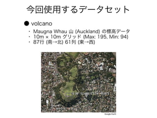
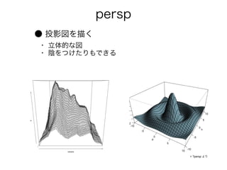
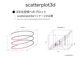
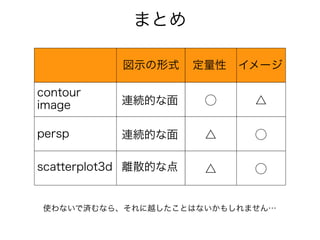
Rを用いて富士山の標高データを3次元グラフとして表現した. contourとimageは連続的な面を描写できるが定量性は低い. perspとscatterplot3dは立体感はあるが点データである. 適切なグラフはデータの性質と目的によって選択されるべきである.

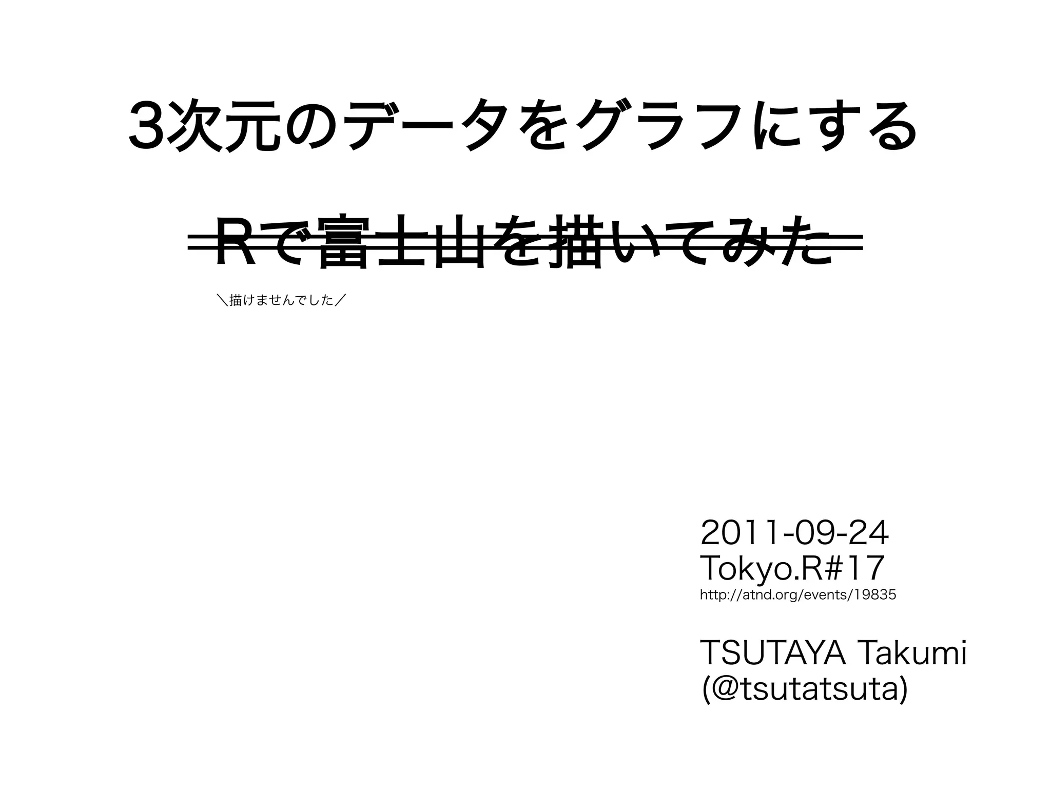
![# データの準備
# データのラベルを作成
south.north <- 1:nrow(volcano) * 10 # rowの数は87
east.west <- 1:ncol(volcano) * 10 # columnの数は61
# 頂上の位置を変数に入れておく
mt.top <- which(volcano == max(volcano), arr.ind = TRUE) * 10
# 標高150mライン
level150 <- which(volcano == 150, arr.ind = TRUE) * 10
# scatterplot3dパッケージの読み込み
library(scatterplot3d)
# http://cran.r-project.org/web/packages/scatterplot3d/index.html
# scatterplot3d用ラベルの準備
south.north.3d <- rep(south.north, length(east.west))
west.east.3d <- vector(length = 87 * 61)
for(i in 1:61){
west.east.3d[((i - 1) * 87 + 1):(i * 87)] <- east.west[i]
}](https://image.slidesharecdn.com/tokyor-v1-1-110923052523-phpapp02/85/3-Tokyo-R-17-6-320.jpg)

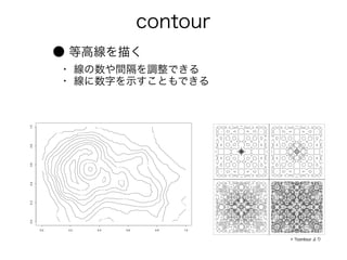
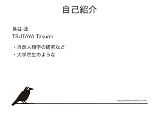
![# 1a # 1b
image(south.north, east.west, volcano, image(south.north, east.west, volcano,
col = terrain.colors(100), col = rainbow(100),
xlab = "South-North", ylab = "East-West") xlab = "South-North", ylab = "East-West")
contour(south.north, east.west, volcano, contour(south.north, east.west, volcano,
levels = c(175, 145), add = TRUE) levels = 160, lty = "dotted", add = TRUE)
points(mt.top[1], mt.top[2], pch = 20, lines(c(0, 1000), c(150, 500))
col = "blue") # 頂上を図示 # (0, 150)と(1000, 150)を通る直線を引く
# 1c # 1d
image(south.north, east.west, volcano, image(south.north, east.west, volcano,
col = gray((10:0)/10), col = gray((0:100)/100),
xlab = "South-North", ylab = "East-West") xlab = "South-North", ylab = "East-West")
contour(south.north, east.west, volcano, contour(south.north, east.west, volcano,
levels = 175, col = "red", add = TRUE) col = rainbow(10), add = TRUE)
points(level150[ , 1], level150[ , 2], pch = 20, text(mt.top[1], mt.top[2], "TOP", col = "blue")
col = "blue") # 標高150mの点を図示 # 頂上に"TOP"をプロット](https://image.slidesharecdn.com/tokyor-v1-1-110923052523-phpapp02/85/3-Tokyo-R-17-11-320.jpg)

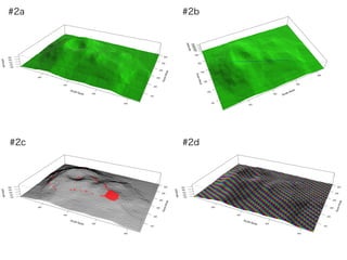
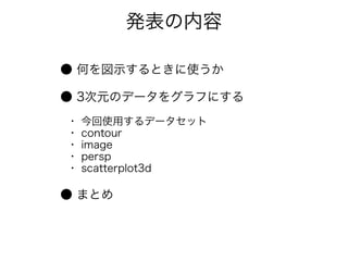
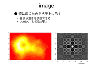
![#2a #2b
mt.mw <- persp(south.north, east.west, mt.mw <- persp(south.north, east.west,
volcano, theta = 25, phi = 30, scale = FALSE, volcano, theta = -25, phi = 50, scale = FALSE,
col = "green", border = NA, ltheta = 120, col = "green", border = NA, ltheta = 120,
shade = 0.7, ticktype = "detailed", shade = 0.5, ticktype = "detailed",
cex.axis = 0.8, xlab = "South-North", cex.axis = 0.8, xlab = "South-North",
ylab = "East-West", zlab = "Altitude") ylab = "East-West", zlab = "Altitude")
points(trans3d(mt.top[1], mt.top[2], max(volcano), x <- 6
pmat = mt.mw), col = "red", pch = 16) lines(trans3d(c(mt.top[1], level150[x, 1]),
# 頂上を図示 c(mt.top[2], level150[x, 2]),
c(max(volcano), 150), pmat = mt.mw), col = "blue")
# 頂上と,標高150mにある一点を結ぶ
#2c #2d
mt.mw <- persp(south.north, east.west, mt.mw <- persp(south.north, east.west,
volcano, theta = 25, phi = 30, scale = FALSE, volcano, theta = 25, phi = 30, scale = FALSE,
col = NA, border = "black", ltheta = 120, col = rainbow(7), border = NA, ltheta = -120,
shade = 0.3, ticktype = "detailed", shade = 0.7, ticktype = "detailed",
cex.axis = 0.8, xlab = "South-North", cex.axis = 0.8, xlab = "South-North",
ylab = "East-West", zlab = "Altitude") ylab = "East-West", zlab = "Altitude")
x <- 6 x <- 6
points(trans3d(level150[ , 1], level150[ , 2], 150, text(trans3d(mt.top[1], mt.top[2], max(volcano),
pmat = mt.mw), col = "red", pch = 16) pmat = mt.mw), "TOP", pch = 16)
# 標高150mの点を図示 # 頂上に"TOP"をプロット](https://image.slidesharecdn.com/tokyor-v1-1-110923052523-phpapp02/85/3-Tokyo-R-17-15-320.jpg)

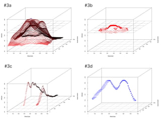
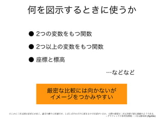
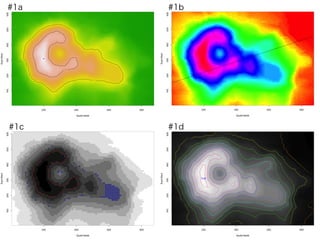
![# 3a # 3b
mt.mw.3d <- scatterplot3d(west.east.3d, level145to150.3d <- which(volcano < 150 &
south.north.3d, volcano, scale.y = 1, volcano >= 145) # 標高145m以上150m未満
highlight.3d = TRUE, level150to155.3d <- which(volcano < 155 &
zlim = c(80, 200), xlab = "West-East", volcano >= 150) # 標高150m以上145m未満
ylab = "South-North", zlab = "Altitude") mt.mw.3d<- scatterplot3d(
mt.mw.3d$plane3d(150, x.coef = 0, y.coef = 0, west.east.3d[level145to150.3d],
lty.box = "dashed") south.north.3d[level145to150.3d],
# 標高150mラインに平面の追加. volcano[level145to150.3d], color = "red",
mt.mw.3d$points3d(mt.top[2], mt.top[1], scale.y = 1, xlim = c(0, 700), ylim = c(0, 1000),
max(volcano), col = "blue", pch = 19) zlim = c(80, 200), xlab = "West-East",
# 頂上の追加. ylab = "South-North", zlab = "Altitude")
mt.mw.3d$plane3d(150, x.coef = 0, y.coef = 0,
lty.box = "dashed") # 標高150mラインに平面
mt.mw.3d$points3d(west.east.3d[level150to155.3d],
south.north.3d[level150to155.3d],
volcano[level150to155.3d], col = "red")
# 標高150m以上155m未満
# 3c
west275to300.3d <- which(west.east.3d < 300 &
west.east.3d >= 275) # 西から275以上300m未満
west500to525.3d <- which(west.east.3d < 525 & # 3d
west.east.3d >= 500) # 西から500以上525m未満 south275to325.3d <- which(south.north.3d < 325 &
label.3d <- c(west275to300.3d, west500to525.3d) south.north.3d >= 275) # 南から275以上325m未満
mt.mw.3d <- scatterplot3d(west.east.3d[label.3d], mt.mw.3d <-scatterplot3d(
south.north.3d[label.3d], volcano[label.3d], west.east.3d[south275to325.3d],
scale.y = 1.5, highlight.3d = TRUE, south.north.3d[south275to325.3d],
xlim = c(0, 700), ylim = c(0, 1000), volcano[south275to325.3d], scale.y = 0.7,
zlim = c(80, 200), xlab = "West-East", color = "blue", xlim = c(0, 700), ylim = c(0, 1000),
ylab = "South-North", zlab = "Altitude") zlim = c(80, 200), xlab = "West-East",
ylab = "South-North", zlab = "Altitude")](https://image.slidesharecdn.com/tokyor-v1-1-110923052523-phpapp02/85/3-Tokyo-R-17-19-320.jpg)


![[研究室論文紹介用スライド] Adversarial Contrastive Estimation](https://cdn.slidesharecdn.com/ss_thumbnails/acepub-181119101425-thumbnail.jpg?width=640&height=640&fit=bounds)


