Download to read offline


![Data processing by dplyr
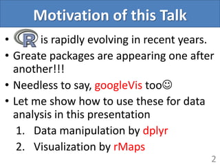
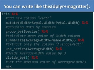
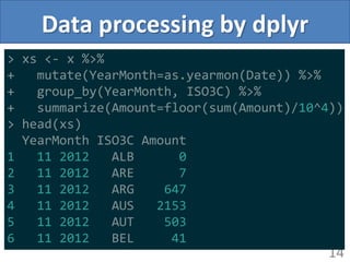
• Define some variables we use later
16
> min.date <- xs %>%
+ use_series(YearMonth) %>%
+ as.Date %>% min %>% as.character
> max.counter <- xs %>%
+ use_series(Counter) %>% max
> min.date
[1] "2012-11-01"
> max.counter
[1] 12](https://image.slidesharecdn.com/globaltokyor120140417-140416075334-phpapp01/85/Trading-volume-mapping-R-in-recent-environment-16-320.jpg)
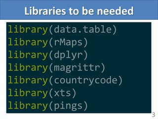
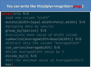
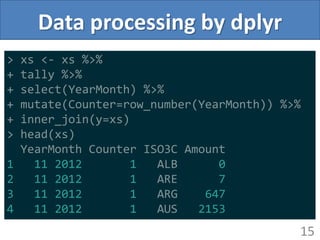
![Visualize with rMaps
19
d <- ichoropleth(log(Amount) ~ ISO3C, data=as.data.frame(xs), animate="Counter", map="world")
d$setTemplate(chartDiv = sprintf("
<div class='container'>
<button ng-click='animateMap()'>Play</button>
<span ng-bind='date_show'></span>
<div id='{{chartId}}' class='rChart datamaps'></div>
</div>
<script src='http://ajax.googleapis.com/ajax/libs/jquery/1/jquery.min.js'></script>
<script src='http://ajax.googleapis.com/ajax/libs/jqueryui/1/jquery-ui.min.js'></script>
<script>
function rChartsCtrl($scope, $timeout){
$scope.counter = 1;
$scope.date = new Date('%s');
$scope.date_show = $.datepicker.formatDate('yy-mm', $scope.date);
$scope.animateMap = function(){
if ($scope.counter > %s){
return;
}
map{{chartId}}.updateChoropleth(chartParams.newData[$scope.counter]);
$scope.counter += 1;
$scope.date.setMonth($scope.date.getMonth()+1);
$scope.date_show = $.datepicker.formatDate('yy-mm', $scope.date);
$timeout($scope.animateMap, 1000)
}
}
</script>", min.date, max.counter)
)
d](https://image.slidesharecdn.com/globaltokyor120140417-140416075334-phpapp01/85/Trading-volume-mapping-R-in-recent-environment-19-320.jpg)
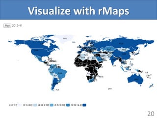


This document discusses visualizing trading volume data using R. It includes: 1. Loading and manipulating trading volume data from 2012 using data.table and dplyr packages to summarize the monthly total trading amount by country. 2. Creating an interactive choropleth map visualization of the monthly trading data over time using the rMaps package. Custom HTML and JavaScript are used to animate the map updating each month. 3. Providing the full codes in a GitHub repository for others to reproduce the analysis and visualization.


![Getting Started with Apache Spark: Big Data Made Simple [Free Meetup]](https://cdn.slidesharecdn.com/ss_thumbnails/apachesparkgettingstarted-260203175547-8361bcc3-thumbnail.jpg?width=640&height=640&fit=bounds)


