Download as PDF, PPTX


![Basic R
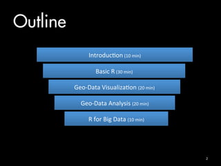
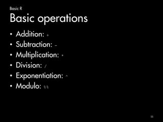
Basic operations
> 1+1 # Addition
[1] 2
> 4 - 3 # Subtraction
[1] 1
> 4 * 2 + 1 # Operator precedence
[1] 9
> 6 ^ 2 # Exponentiation
[1] 36
> sqrt(5) # Math function
[1] 2.236068
12](https://image.slidesharecdn.com/bigdatacourse-141008143905-conversion-gate01/85/Big-datacourse-12-320.jpg)
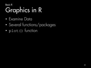
![Basic R
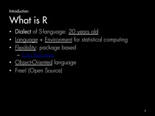
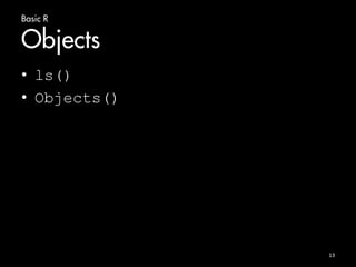
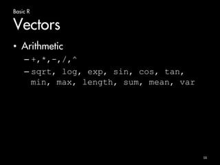
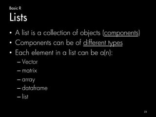
Vectors
• Sequence
17
> 1:10
[1] 1 2 3 4 5 6 7 8 9 10
> 10:1
[1] 10 9 8 7 6 5 4 3 2 1
> seq(from = 1, to = 10)
[1] 1 2 3 4 5 6 7 8 9 10
> seq(from = 10, to = 1)
[1] 10 9 8 7 6 5 4 3 2 1
> seq(from = 1, length = 10, by =4)
[1] 1 5 9 13 17 21 25 29 33 37](https://image.slidesharecdn.com/bigdatacourse-141008143905-conversion-gate01/85/Big-datacourse-17-320.jpg)
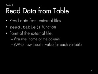
![Basic R
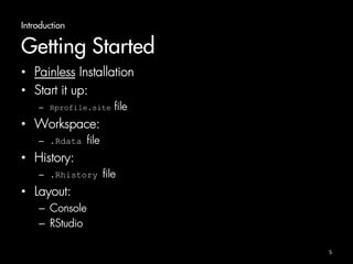
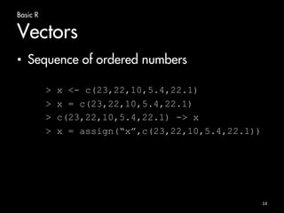
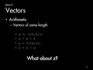
Vectors
• Logical vectors
> x = seq(from=1, to=10)
> x
[1] 1 2 3 4 5 6 7 8 9 10
> y = (x %% 3 == 0)
> y
[1] FALSE FALSE TRUE FALSE FALSE TRUE
FALSE FALSE TRUE FALSE
18](https://image.slidesharecdn.com/bigdatacourse-141008143905-conversion-gate01/85/Big-datacourse-18-320.jpg)
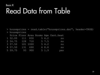
![Basic R
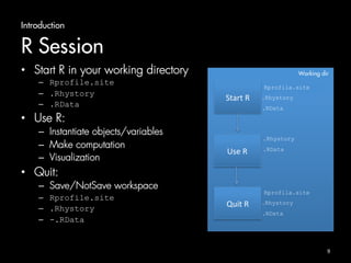
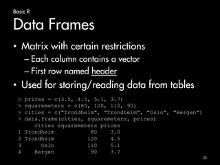
Vectors
• Index vectors
– Access by index
– From 1
– Logical condition
19
> x = c(2,5,7,9)
> x[1]
[1] 2
> x[c(2,4)]
[1] 5 9
> x[x<7]
[1] 2 5](https://image.slidesharecdn.com/bigdatacourse-141008143905-conversion-gate01/85/Big-datacourse-19-320.jpg)
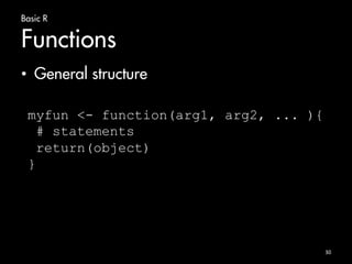
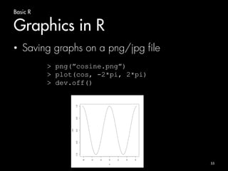
![Basic R
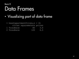
Arrays and Matrices in R
• Matrix
– A matrix is a two-dimensional object
– matrix function
20
> matrixA = matrix(data = c(1:10), ncol = 2, nrow = 5)
> matrixA
[,1] [,2]
[1,] 1 6
[2,] 2 7
[3,] 3 8
[4,] 4 9
[5,] 5 10](https://image.slidesharecdn.com/bigdatacourse-141008143905-conversion-gate01/85/Big-datacourse-20-320.jpg)
![Basic R
Arrays and Matrices in R
• Array
– A matrix is a n-dimensional object
– array function + dim
> x = c(1:18)
> x
[1] 1 2 3 4 5 6 7 8 9 10 11 12 13 14 15 16 17 18
> y = array(data=x, dim=c(2,3,3))
21](https://image.slidesharecdn.com/bigdatacourse-141008143905-conversion-gate01/85/Big-datacourse-21-320.jpg)
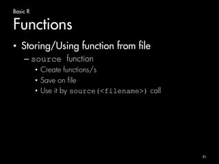
![Basic R
Arrays and Matrices in R
• Accessing by index
22
> x <- array(data=c(1:12), dim=c(3,4)) #generate 3 by 4 matrix
> x
[,1] [,2] [,3] [,4]
[1,] 1 4 7 10
[2,] 2 5 8 11
[3,] 3 6 9 12
> i <- array(c(1:3,3:1), dim=c(3,2))
> i
> [,1] [,2]
> [1,] 1 3
> [2,] 2 2
> [3,] 3 1
> x[i]
[1] 7 5 3
> x[i] <- -1
> x
[,1] [,2] [,3] [,4]
[1,] 1 4 -1 10
[2,] 2 -1 8 11
[3,] -1 6 9 12](https://image.slidesharecdn.com/bigdatacourse-141008143905-conversion-gate01/85/Big-datacourse-22-320.jpg)
![Basic R
Lists
• Example:
24
> lst = list(name="Massimiliano", surname="Ruocco",
> age=99, birthplace="Italy")
> lst$name
[1] "Massimiliano”
> lst[1]
$name
[1] "Massimiliano"](https://image.slidesharecdn.com/bigdatacourse-141008143905-conversion-gate01/85/Big-datacourse-24-320.jpg)
![Basic R
Data Frames
• Accessing as a normal matrix
26
> apartmentPrices[2,1]
[1] Trondheim
Levels: Bergen Oslo Trondheim
> apartmentPrices[1,]
cities squaremeters prices
1 Trondheim 80 3
> apartmentPrices$prices
[1] 3.0 4.5 5.1 3.7](https://image.slidesharecdn.com/bigdatacourse-141008143905-conversion-gate01/85/Big-datacourse-26-320.jpg)


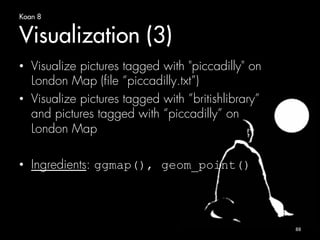
![Koan 3
Basic R (2)
• create a vector with only odd numbers
from 1 to 100
• create a vector [1,2,3,...,100]. Extract
from this the vector with only odd
numbers
• Compare the two resulting vectors
78](https://image.slidesharecdn.com/bigdatacourse-141008143905-conversion-gate01/85/Big-datacourse-79-320.jpg)


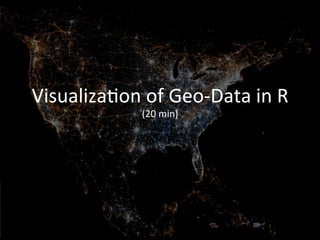
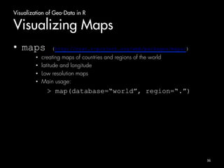
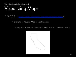
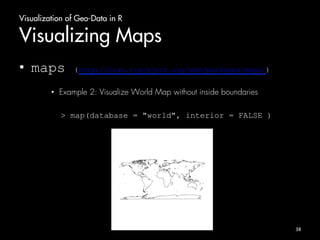
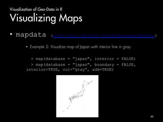
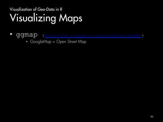
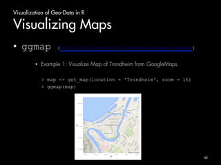
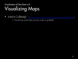
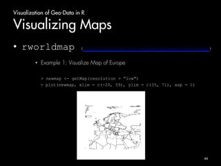
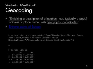
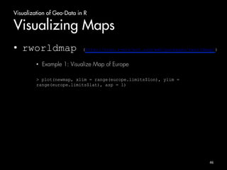
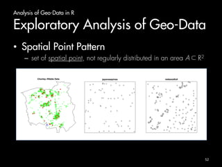
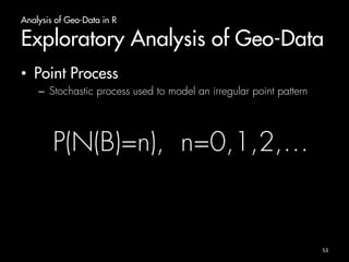
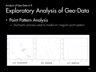
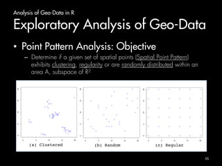
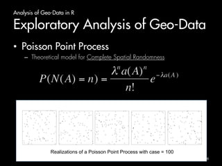
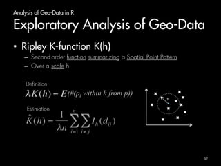
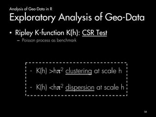
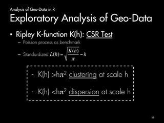
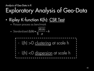
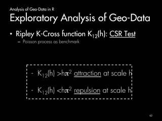
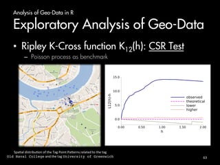
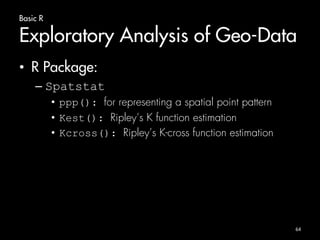
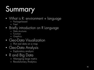
The document outlines an introduction to analyzing and visualizing geo-data in R. It discusses exploring the structure of spatially distributed point data through point process statistics like the Complete Spatial Randomness test and Ripley's K-function. It also covers visualizing maps and point patterns with packages like maps, ggmap, rworldmap, and ggplot2. The document provides examples of mapping different regions, geocoding location data, and plotting point patterns on maps in R.


![[Paper Reading] Generalized Sub-Query Fusion for Eliminating Redundant I/O fr...](https://cdn.slidesharecdn.com/ss_thumbnails/resin-210920113222-thumbnail.jpg?width=640&height=640&fit=bounds)


![제 23회 보아즈(BOAZ) 빅데이터 컨퍼런스 - [MBOAX] : ABSA를 활용한 소비자 반응 분석 기반 운영 효율화 대시보드 설계](https://cdn.slidesharecdn.com/ss_thumbnails/3-1boaz23rdconferencemboax-260203102709-9d519923-thumbnail.jpg?width=640&height=640&fit=bounds)


