SlideShare a Scribd company logo
1 of 87
Download to read offline
Unit 3: Classification LH 7
Presented By : Tekendra Nath Yogi
Tekendranath@gmail.com
College Of Applied Business And Technology
Contd…
• Outline:
– 3.1. Basics
– 3.2. Decision Tree Classifier
– 3.3. Rule Based Classifier
– 3.4. Nearest Neighbor Classifier
– 3.5. Bayesian Classifier
– 3.6. Artificial Neural Network Classifier
– 3.7. Issues : Over-fitting, Validation, Model Comparison
26/19/2019 By: Tekendra Nath Yogi
June 19, 2019 By:Tekendra Nath Yogi 3
Introduction
• Databases are rich with hidden information that can be used for intelligent
decision making.
• Classification and prediction are two forms of data analysis that can be used to
extract models describing important data classes or to predict future data
trends. Such analysis provide better understanding of the data at large.
• classification predicts categorical (discrete, unordered) labels, prediction
models continuous valued functions i.e., predicts unknown or missing values.
June 19, 2019 By:Tekendra Nath Yogi 4
Contd…
• When to use classification?
– Following are the examples of cases where the data analysis task is
Classification :
• A bank loan officer wants to analyze the data in order to know which
customer (loan applicant) are risky or which are safe.
• A marketing manager at a company needs to analyze a customer with
a given profile, who will buy a new computer.
– In both of the above examples, a model or classifier is constructed to
predict the categorical labels. These labels are risky or safe for loan
application data and yes or no for marketing data.
June 19, 2019 By:Tekendra Nath Yogi 5
Contd…
• When to use Prediction?
– Following are the examples of cases where the data analysis task is
Prediction :
• Suppose the marketing manager needs to predict how much a given
customer will spend during a sale at his company.
• In this example we are bothered to predict a numeric value. Therefore
the data analysis task is an example of numeric prediction.
• In this case, a model or a predictor will be constructed that predicts a
continuous value.
June 19, 2019 By:Tekendra Nath Yogi 6
How does classification work?
• The Data Classification process includes two steps:
– Building the Classifier or Model
– Using Classifier for Classification
June 19, 2019 By:Tekendra Nath Yogi 7
Contd…
• Building the Classifier or Model:
– Also known as model construction, training or learning phase
– a classification algorithm builds the classifier (e.g., decision tree, if-then
rules or mathematical formulae and etc) by analyzing or ―learning from‖ a
training set made up of database tuples and their associated class labels.
– Because the class label of each training tuple is provided, this step is also
known as supervised learning
– i.e., the learning of the classifier is ―supervised‖ in that it is told to which
class each training tuple belongs.
June 19, 2019 By:Tekendra Nath Yogi 8
Contd…
• E.g.,
June 19, 2019 By:Tekendra Nath Yogi 9
Contd…
• Using Classifier for Classification: Before using the model, we first
need to test its accuracy
• Measuring model accuracy:
– To measure the accuracy of a model we need test data (randomly selected
from the general data set.)
– Test data is similar in its structure to training data (labeled data)
– How to test?
– The known label of test sample is compared with the classified result from
the model
– Accuracy rate is the percentage of test set samples that are correctly
classified by the model
– Important: test data should be independent of training set, otherwise over-
fitting will occur
• Using the model: If the accuracy is acceptable, use the model to classify data
tuples whose class labels are not known
casestestofnumberTotal
tionsclassificacorrectofNumber
Accuracy
June 19, 2019 By:Tekendra Nath Yogi 10
Contd…
• E.g.,:
• Here, Accuracy =3/4*100=75%
June 19, 2019 By:Tekendra Nath Yogi 11
Contd…
• Example to illustrate the steps of classification:
– Model construction:
June 19, 2019 By:Tekendra Nath Yogi 12
Contd…
• Model Usage:
Big spenders
Classification by Decision Tree Induction
• Decision tree induction is the learning of decision trees from class labeled
training tuples
• Decision tree is A flow-chart-like tree structure
– Internal node denotes a test on an attribute
– Branch represents an outcome of the test
– Leaf nodes represent class labels or class distribution
June 19, 2019 13By:Tekendra Nath Yogi
June 19, 2019 By:Tekendra Nath Yogi 14
Contd…
• How are decision trees used for classification?
– The attributes of a tuple are tested against the decision tree
– A path is traced from the root to a leaf node which holds the prediction for
that tuple
June 19, 2019 By:Tekendra Nath Yogi 15
Contd…
Algorithm for Decision Tree Induction
• Basic algorithm (a greedy algorithm)
– At start, all the training examples are at the root
– Samples are partitioned recursively based on selected attributes called
the test attributes.
– Test attributes are selected on the basis of a heuristic or statistical
measure (e.g., information gain)
• Conditions for stopping partitioning
– All samples for a given node belong to the same class
– There are no remaining attributes for further partitioning – majority
voting is employed for classifying the leaf
– There are no samples left
June 19, 2019 16By:Tekendra Nath Yogi
Algorithm for Decision Tree Induction (pseudocode)
Algorithm GenDecTree(Sample S, Attlist A)
1. create a node N
2. If all samples are of the same class C then label N with C; terminate;
3. If A is empty then label N with the most common class C in S (majority
voting); terminate;
4. Select aA, with the highest information gain; Label N with a;
5. For each value v of a:
a. Grow a branch from N with condition a=v;
b. Let Sv be the subset of samples in S with a=v;
c. If Sv is empty then attach a leaf labeled with the most common class in S;
d. Else attach the node generated by GenDecTree(Sv, A-a)
June 19, 2019 17By:Tekendra Nath Yogi
June 19, 2019 By:Tekendra Nath Yogi 18
Contd…
• E.g.,
June 19, 2019 By:Tekendra Nath Yogi 19
Contd…
June 19, 2019 By:Tekendra Nath Yogi 20
Contd…
June 19, 2019 By:Tekendra Nath Yogi 21
Contd…
June 19, 2019 By:Tekendra Nath Yogi 22
Contd…
June 19, 2019 By:Tekendra Nath Yogi 23
Contd…
June 19, 2019 By:Tekendra Nath Yogi 24
Contd…
June 19, 2019 By:Tekendra Nath Yogi 25
Attribute Selection Measures
• An attribute selection measure is a heuristic for selecting the splitting criterion
that ―best‖ separates a given data partition D
• splitting rules
– Provide ranking for each attribute describing the tuples
– The attribute with highest score is chosen
• Methods
– Information gain
– Gain ratio
– Gini Index
June 19, 2019 By:Tekendra Nath Yogi 26
Contd…
• 1st approach: Information Gain Approach:
– D: the current partition
– N: represent the tuples of partition D
– Select the attribute with the highest information gain
– This attribute
• minimizes the information needed to classify the tuples in the
resulting partitions
• reflects the least randomness or ―impurity‖ in these partitions
– Information gain approach minimizes the expected number of tests needed
to classify a given tuple and guarantees a simple tree
June 19, 2019 By:Tekendra Nath Yogi 27
Contd…
• Let pi be the probability that an arbitrary tuple in D (data set) belongs to class
Ci, estimated by |Ci, D|/|D|
 Expected information needed to classify a tuple in D:
 Information needed (after using A to split D into v partitions) to classify D:
 Information gained by branching on attribute A:
)(log)( 2
1
i
m
i
i ppDInfo 

)(
||
||
)(
1
j
v
j
j
A DI
D
D
DInfo  
(D)InfoInfo(D)Gain(A) A
m: the number of classes
June 19, 2019 By:Tekendra Nath Yogi 28
Contd…
• Expected information needed to classify a tuple in D:
)(log)( 2
1
i
m
i
i ppDInfo 

June 19, 2019 By:Tekendra Nath Yogi 29
Contd…
• Information needed (after using A to split D into v partitions) to
classify D: )(
||
||
)(
1
j
v
j
j
A DI
D
D
DInfo  
June 19, 2019 By:Tekendra Nath Yogi 30
Contd…
• Information gained by branching on attribute A: (D)InfoInfo(D)Gain(A) A
Contd…
income student credit_rating buys_computer
high no fair no
high no excellent no
medium no fair no
low yes fair yes
medium yes excellent yes
income student credit_rating buys_computer
high no fair yes
low yes excellent yes
medium no excellent yes
high yes fair yes
income student credit_rating buys_computer
medium no fair yes
low yes fair yes
low yes excellent no
medium yes fair yes
medium no excellent no
age?
Youth
Middle aged
Senior
labeled yes
• Because age has the highest information gain among the attributes, it is
selected as the splitting attribute
June 19, 2019 31By:Tekendra Nath Yogi
Contd….
age?
overcast
student? credit rating?
no yes fairexcellent
youth senior
no noyes yes
yes
Middle aged
June 19, 2019 32By:Tekendra Nath Yogi
Output: A Decision Tree for ―buys_computer
Similarly,
Contd…
• Decision Tree Based Classification of Advantages:
– Inexpensive to construct
– Extremely fast at classifying unknown records
– Easy to interpret for small-sized trees
– Robust to noise (especially when methods to avoid over-fitting are
employed)
– Can easily handle redundant or irrelevant attributes (unless the
attributes are interacting)
June 19, 2019 33By:Tekendra Nath Yogi
Contd…
• Decision Tree Based Classification Disadvantages:
– Space of possible decision trees is exponentially large. Greedy
approaches are often unable to find the best tree.
– Does not take into account interactions between attributes
– Each decision boundary involves only a single attribute
June 19, 2019 34By:Tekendra Nath Yogi
June 19, 2019 By:Tekendra Nath Yogi 35
Naïve Bayes Classification
• Bayesian classifiers are statistical classifiers. They can predict class
membership probabilities, such as the probability that a given tuple belongs to
a particular class.
• i.e., For each new sample they provide a probability that the sample belongs to
a class (for all classes).
• Based on Bayes‘ Theorem
June 19, 2019 By:Tekendra Nath Yogi 36
Contd…
• Bayes‘ Theorem :
– Given the training data set D and data sample to be classified X whose
class label is unknown.
– Let H be a hypothesis that X belongs to class C
– Classification is to determine P(H|X), the probability that the hypothesis
holds given the observed data sample X.
– Predicts X belongs to Class Ci iff the probability P(Ci|X) is the highest
among all the P(Ck|X) for all the k classes.
– P(H), P(X|H), and P(X) can be estimated from the given data set.
)(
)()|()|(
X
XX
P
HPHPHP 
June 19, 2019 By:Tekendra Nath Yogi 37
Contd…
• The naïve Bayesian classifier, or simple Bayesian classifier,
works as follows:
1. Let D be a training set of tuples and their associated class labels and
X={x1, x2,…..xK} be a tuple that is to be classified based on D. i.e.,
unlabelled data whose class label is to be find.
2. In order to predict the class label of X, perform the following calculations
for each class ci .
a. Calculate Probability of each class ci as: P(Ci)=|Ci, D|/|D|, where |Ci, D|
is the number of training tuples of class Ci in D.
June 19, 2019 By:Tekendra Nath Yogi 38
Contd…
b) For each value of attributes in X calculate P(xk|Ci)As:
c) Calculate the Probalility of a tuple X conditioned on class Ci as:
d) Calculate the probalility of class ci , conditioned on X as:
P(Ci|X)= P(X|Ci)*P(Ci).
3. predict the class label of X as: The predicted class label of X is the class Ci for
which P(X|Ci)*P(Ci) is the maximum.
)|(...)|()|(
1
)|()|(
21
CixPCixPCixP
n
k
CixPCiP
nk


X
DinCiclassoftuplesofnumberthe|,DCi,|
AkattributeforxkvaluethehavingDinCiclassoftuples#
Ci)|P(xk 
June 19, 2019 By:Tekendra Nath Yogi 39
Contd…
• Example: study the training data given below and construct a Naïve Bayes
classifier and then classify the given sample.
• Training set:
• classify a new sample X = (age <= 30 , income = medium, student = yes, credit_rating = fair)
age income studentcredit_ratingbuys_computer
<=30 high no fair no
<=30 high no excellent no
31…40 high no fair yes
>40 medium no fair yes
>40 low yes fair yes
>40 low yes excellent no
31…40 low yes excellent yes
<=30 medium no fair no
<=30 low yes fair yes
>40 medium yes fair yes
<=30 medium yes excellent yes
31…40 medium no excellent yes
31…40 high yes fair yes
>40 medium no excellent no
June 19, 2019 By:Tekendra Nath Yogi 40
Contd…
• Solution: In the given training data set two classes yes and no are present.
– Let, C1:buys_computer = ‗yes‘ and C2:buys_computer = ‗no‘
• Calculate Probability of each class ci as: P(Ci)=|Ci, D|/|D|, where |Ci, D| is the
number of training tuples of class Ci in D.
– P(buys_computer = ―yes‖) = 9/14 = 0.643
– P(buys_computer = ―no‖) = 5/14= 0.357
age income studentcredit_ratingbuys_compute
<=30 high no fair no
<=30 high no excellent no
31…40 high no fair yes
>40 medium no fair yes
>40 low yes fair yes
>40 low yes excellent no
31…40 low yes excellent yes
<=30 medium no fair no
<=30 low yes fair yes
>40 medium yes fair yes
<=30 medium yes excellent yes
31…40 medium no excellent yes
31…40 high yes fair yes
>40 medium no excellent no
June 19, 2019 By:Tekendra Nath Yogi 41
Contd…
• Compute P(XK|Ci) for each class:
P(age = ―<=30‖ | buys_computer = ―yes‖) = 2/9 = 0.222
P(age = ―<= 30‖ | buys_computer = ―no‖) = 3/5 = 0.6
P(income = ―medium‖ | buys_computer = ―yes‖) = 4/9 = 0.444
P(income = ―medium‖ | buys_computer = ―no‖) = 2/5 = 0.4
P(student = ―yes‖ | buys_computer = ―yes) = 6/9 = 0.667
P(student = ―yes‖ | buys_computer = ―no‖) = 1/5 = 0.2
P(credit_rating = ―fair‖ | buys_computer = ―yes‖) = 6/9 = 0.667
P(credit_rating = ―fair‖ | buys_computer = ―no‖) = 2/5 = 0.4
June 19, 2019 By:Tekendra Nath Yogi 42
Contd…
• Compute P(X|Ci) for each class:
– P(X|buys_computer = ―yes‖) = 0.222 x 0.444 x 0.667 x 0.667 = 0.044
– P(X|buys_computer = ―no‖) = 0.6 x 0.4 x 0.2 x 0.4 = 0.019
• Calculate the probalility of class ci , conditioned on X as: P(Ci|X)=P(X|Ci)*P(Ci)
– P(buys_computer = ―yes‖ | X ) =P(X|buys_computer = ―yes‖) * P(buys_computer
= ―yes‖) = 0.028 (maximum).
– P(buys_computer = ―no‖ |X) = P(X|buys_computer = ―no‖) * P(buys_computer =
―no‖) = 0.007
• Therefore, X belongs to class (“buys_computer = yes”)
43
Contd…
• Avoiding the 0-Probability Problem:
– Naïve Bayesian prediction requires each conditional prob. be non-zero.
Otherwise, the predicted prob. will be zero
– Ex. Suppose a dataset with 1000 tuples, income=low (0), income= medium
(990), and income = high (10),
– Use Laplacian correction
• Adding 1 to each case
Prob(income = low) = 1/1003
Prob(income = medium) = 991/1003
Prob(income = high) = 11/1003
• The ―corrected‖ prob. estimates are close to their ―uncorrected‖ counterparts



n
k
CixkPCiXP
1
)|()|(
June 19, 2019 By:Tekendra Nath Yogi
44
Contd…
• Advantages
– Easy to implement
– Good results obtained in most of the cases
• Disadvantages
– Assumption: class conditional independence, therefore loss of
accuracy
– Practically, dependencies exist among variables
• E.g., hospitals: patients: Profile: age, family history, etc.
Symptoms: fever, cough etc., Disease: lung cancer, diabetes, etc.
• Dependencies among these cannot be modeled by Naïve Bayesian
Classifier
June 19, 2019 By:Tekendra Nath Yogi
June 19, 2019 By:Tekendra Nath Yogi 45
Contd…
• Example: study the training data given below and construct a Naïve Bayes
classifier and then classify the given sample.
• Training set:
• classify a new sample X:< outlook = sunny, temperature = cool, humidity =
high, windy = false>
Outlook Temperature Humidity Windy Class
sunny hot high false N
sunny hot high true N
overcast hot high false P
rain mild high false P
rain cool normal false P
rain cool normal true N
overcast cool normal true P
sunny mild high false N
sunny cool normal false P
rain mild normal false P
sunny mild normal true P
overcast mild high true P
overcast hot normal false P
rain mild high true N
play tennis?
June 19, 2019 By:Tekendra Nath Yogi 46
Contd…
• Solution:
Outlook Temperature Humidity Windy Class
sunny hot high false N
sunny hot high true N
rain cool normal true N
sunny mild high false N
rain mild high true N
Outlook Temperature Humidity Windy Class
overcast hot high false P
rain mild high false P
rain cool normal false P
overcast cool normal true P
sunny cool normal false P
rain mild normal false P
sunny mild normal true P
overcast mild high true P
overcast hot normal false P
9
5
June 19, 2019 By:Tekendra Nath Yogi 47
Contd…
• Given the training set, we compute the probabilities:
• We also have the probabilities
– P = 9/14
– N = 5/14
O utlook P N Hum idity P N
sunny 2/9 3/5 high 3/9 4/5
overcast 4/9 0 norm al 6/9 1/5
rain 3/9 2/5
Tem preature W indy
hot 2/9 2/5 true 3/9 3/5
m ild 4/9 2/5 false 6/9 2/5
cool 3/9 1/5
June 19, 2019 By:Tekendra Nath Yogi 48
Contd…
• To classify a new sample X: < outlook = sunny, temperature = cool, humidity =
high, windy = false>
• Prob(P|X) = Prob(P)*Prob(sunny|P)*Prob(cool|P)* Prob(high|P)*Prob(false|P)
= 9/14*2/9*3/9*3/9*6/9 = 0.01
• Prob(N|X) =Prob(N)*Prob(sunny|N)*Prob(cool|N)*Prob(high|N)*Prob(false|N)
= 5/14*3/5*1/5*4/5*2/5 = 0.013
• Therefore X takes class label N
Artificial Neural Network
• A neural network is composed of number of nodes or units , connected by
links. Each link has a numeric weight associated with it.
• Actually artificial neural networks are programs design to solve any problem
by trying to mimic the structure and the function of our nervous system.
496/19/2019 Presented By: Tekendra Nath Yogi
2
1
3
4
5
6
Input
Layer
Hidden
Layer Output
Layer
Artificial neural network model:
• Input to the network are represented by mathematical symbol xn.
• Each of these inputs are multiplied by a connection weight, wn
• These products are simply summed, fed through the transfer function f() to
generate result and output
50
nnxwxwxwsum  ......2211
6/19/2019 Presented By: Tekendra Nath Yogi
Back propagation algorithm
• Back propagation is a neural network learning algorithm. Learns by
adjusting the weight so as to be able to predict the correct class label of
the input.
Input: D training data set and their associated class label
l= learning rate(normally 0.0-1.0)
Output: a trained neural network.
Method:
Step1: initialize all weights and bias in network.
Step2: while termination condition is not satisfied .
For each training tuple x in D
516/19/2019 Presented By: Tekendra Nath Yogi
2.1 calculate output:
For input layer
For hidden layer and output layer
52
jj IO 
e
j
j
jkjk
I
k
j
O
WOI



 
1
1
* 
Contd…
6/19/2019 Presented By: Tekendra Nath Yogi
2.2 Calculate error:
For output layer:
For hidden layer:
2.3 Update weight
2.4 Update bias
53
))(1( jjjjj OOOerr  
)*()1( 
k
jkkjjj WerrOOerr
jiijij errOloldWnewW **)()( 
jjj errl *
Contd…
6/19/2019 Presented By: Tekendra Nath Yogi
6/19/2019 Presented By: Tekendra Nath Yogi 54
Contd…
• Example: Sample calculations for learning by the back-propagation algorithm.
• Figure above shows a multilayer feed-forward neural network. Let the
learning rate be 0.9. The initial weight and bias values of the network are
given in Table below, along with the first training tuple, X = (1, 0, 1), whose
class label is 1.
1
6/19/2019 Presented By: Tekendra Nath Yogi 55
Contd…
• Step1: Initialization
– Let initial input weight and bias values are:
– Initial input:
– Bias values:
– Initial weight:
X1 X2 X3
1 0 1
-0.4 0.2 0.1
4
W14 W15 W24 W25 W34 W35 W46 W56
0.2 -0.3 0.4 0.1 -0.5 0.2 -0.3 -0.2
5 6
6/19/2019 Presented By: Tekendra Nath Yogi 56
Contd…
• 2. Termination condition: Weight of two successive iteration are nearly
equal or user defined number of iterations are reached.
• 2.1For each training tuple X in D, calculate the output for each input layer:
– For input layer:
• O1=I1=1
• O2=I2=0
• O3=I3=1
jj IO 
6/19/2019 Presented By: Tekendra Nath Yogi 57
Contd…
• For hidden layer and output layer:
1.
2.
332.0
)7182.2(1
1
1
1
1
1
0.7-
(-0.5)*10.4*00.2*1
4W34*O3W24*O2W14*O1
)7.0()7.0(4
4
4










 
ee
I
O
I 
525.0
)7182.2(1
1
1
1
1
1
0.1
0.2*10.1*0(-0.3)*1
5W35*O3W25*O2W15*O1
)1.0()1.0(5
5
5











ee
I
O
I 
6/19/2019 Presented By: Tekendra Nath Yogi 58
Contd…
3.
474.0
)7182.2(1
1
1
1
1
1
0.105-
0.1*1(-0.2)*0.5250.3)(*332.0
5W56*O5W46*O4
)105.0()105.0(6
6
6










 

ee
I
O
I 
6/19/2019 Presented By: Tekendra Nath Yogi 59
Contd…
• Calculation of error at each node:
• For output layer:
• For Hidden layer:
1311.0)474.01)(474.01(474.0
))(1(
))(1(
66666



OOOerr
OOOerr jjjjj


0087.0
))3.0(*1311.0)(332.01(332.0
)*)(1(
)*)(1(
0065.0
))2.0(*1311.0)(525.01(525.0
)*)(1(
)*)(1(
)*()1(
46644
56655








 
WerrOO
WerrOOerr
WerrOO
WerrOOerr
WerrOOerr
•
jkkjjj
•
jkkjjj
jkkjjj
k
6/19/2019 Presented By: Tekendra Nath Yogi 60
Contd…
• Update the weight:
1.
2.
3.
jiijij errOloldWnewW **)()( 
26.0
332.0*1311.0*9.03.0
**)()( 644646


 errOloldWnewW
138.0
525.0*1311.0*9.02.0
**)()( 655656


 errOloldWnewW
192.0
1*0087.0*9.02.0
**)()( 411414


 errOloldWnewW
6/19/2019 Presented By: Tekendra Nath Yogi 61
Contd…
4.
5.
6.
4.0
0*0087.0(*9.04.0
**)()( 422424


 errOloldWnewW
306.0
1*)0065.0(*9.03.0
**)()( 511515


 errOloldWnewW
508.0
1*0087.0(*9.05.0
**)()( 433434


 errOloldWnewW
6/19/2019 Presented By: Tekendra Nath Yogi 62
Contd…
7.
8.
194.0
1*)0065.0(*9.02.0
**)()( 533535


 errOloldWnewW
1.0
0*)0065.0(*9.01.0
**)()( 522525


 errOloldWnewW
6/19/2019 Presented By: Tekendra Nath Yogi 63
Contd…
• Update the Bias value:
1.
2.
3. And so on until convergence!
jjj errl *
218.0
1311.0*9.01.0
* 6)(66


 errlold
195.0
)0065.0(*9.02.0
* 5)(55


 errlold
408.0
)0087.0(*9.0)4.0(
* 4)(46


 errlold
Rule Based Classifier
• In Rule based classifiers learned model is represented as a set of If-Then
rules.
• A rule-based classifier uses a set of IF-THEN rules for classification.
• An IF-THEN rule is an expression of the form
– IF condition THEN conclusion.
– An example is : IF(Give Birth = no)  (Can Fly = yes) THEN Birds
• The ―IF‖ part (or left side) of a rule is known as the rule antecedent or
precondition.
• The ―THEN‖ part (or right side) is the rule consequent. In the rule antecedent,
the condition consists of one or more attribute tests (e.g., (Give Birth = no) 
(Can Fly = yes)) That are logically ANDed. The rule‘s consequent contains a
class prediction.
May 20, 2018 64By: Tekendra Nath Yogi
Contd..
• Rule-based Classifier (Example)
May 20, 2018 65By: Tekendra Nath Yogi
Name Blood Type Give Birth Can Fly Live in Water Class
human warm yes no no mammals
python cold no no no reptiles
salmon cold no no yes fishes
whale warm yes no yes mammals
frog cold no no sometimes amphibians
komodo cold no no no reptiles
bat warm yes yes no mammals
pigeon warm no yes no birds
cat warm yes no no mammals
leopard shark cold yes no yes fishes
turtle cold no no sometimes reptiles
penguin warm no no sometimes birds
porcupine warm yes no no mammals
eel cold no no yes fishes
salamander cold no no sometimes amphibians
gila monster cold no no no reptiles
platypus warm no no no mammals
owl warm no yes no birds
dolphin warm yes no yes mammals
eagle warm no yes no birds
R1: (Give Birth = no)  (Can Fly = yes)  Birds
R2: (Give Birth = no)  (Live in Water = yes)  Fishes
R3: (Give Birth = yes)  (Blood Type = warm)  Mammals
R4: (Give Birth = no)  (Can Fly = no)  Reptiles
R5: (Live in Water = sometimes)  Amphibians
How does Rule-based Classifier Work?
R1: (Give Birth = no)  (Can Fly = yes)  Birds
R2: (Give Birth = no)  (Live in Water = yes)  Fishes
R3: (Give Birth = yes)  (Blood Type = warm)  Mammals
R4: (Give Birth = no)  (Can Fly = no)  Reptiles
R5: (Live in Water = sometimes)  Amphibians
A lemur triggers rule R3, so it is classified as a mammal
A turtle triggers both R4 and R5
A dogfish shark triggers none of the rules
Name Blood Type Give Birth Can Fly Live in Water Class
lemur warm yes no no ?
turtle cold no no sometimes ?
dogfish shark cold yes no yes ?
May 20, 2018 66By: Tekendra Nath Yogi
May 20, 2018 By: Tekendra Nath Yogi 67
age?
student? credit rating?
<=30 >40
no yes yes
yes
31..40
fairexcellentyesno
• Example: Rule extraction from our buys_computer decision-tree
IF age = young AND student = no THEN buys_computer = no
IF age = young AND student = yes THEN buys_computer = yes
IF age = mid-age THEN buys_computer = yes
IF age = old AND credit_rating = excellent THEN buys_computer = yes
IF age = young AND credit_rating = fair THEN buys_computer = no
Rule Extraction from a Decision Tree
 Rules are easier to understand than large trees
 One rule is created for each path from the root to a
leaf
 Each attribute-value pair along a path forms a
conjunction: the leaf holds the class prediction
Rule Coverage and Accuracy
• A Rule R can be assessed by its
coverage and accuracy
• Coverage of a rule:
– Fraction of records that satisfy the
antecedent of a rule
• Accuracy of a rule:
– Fraction of records that satisfy the
antecedent that also satisfy the
consequent of a rule
Tid Refund Marital
Status
Taxable
Income Class
1 Yes Single 125K No
2 No Married 100K No
3 No Single 70K No
4 Yes Married 120K No
5 No Divorced 95K Yes
6 No Married 60K No
7 Yes Divorced 220K No
8 No Single 85K Yes
9 No Married 75K No
10 No Single 90K Yes
10
(Status=Single)  No
Coverage = 40%, Accuracy = 50%
May 20, 2018 68By: Tekendra Nath Yogi
Contd..
• Advantages of Rule-Based Classifiers:
– As highly expressive as decision trees
– Easy to interpret
– Easy to generate
– Can classify new instances rapidly
– Performance comparable to decision trees
May 20, 2018 69By: Tekendra Nath Yogi
K-Nearest Neighbor (KNN) Classifier
• KNN is a non-parametric, lazy learning algorithm.
• non-parametric:
– means that it does not make any assumptions on the underlying data
distribution.
– Therefore, KNN used when there is little or no prior knowledge about
the data distribution.
• Lazy:
– means that it does not have explicit training phase or it is very
minimal.
June 19, 2019 70By: Tekendra Nath Yogi
Contd….
• KNN stores the entire training dataset which it uses as its representation.
i.e., KNN does not learn any model.
• A positive integer k ( number of nearest neighbors) is specified, along with
a new sample X.
• KNN makes predictions just-in-time by calculating the similarity between
an input sample and each training instance.
• We select the k entries in our training data set which are closest to the new
sample
• We find the most common classification of these entries ( majority voting).
• This is the classification we give to the new sample
June 19, 2019 71By: Tekendra Nath Yogi
Contd….
June 19, 2019 72By: Tekendra Nath Yogi
Contd….
• KNN Algorithm:
– Read the training data D, data sample to be classified X and the value
of k ( number of nearest neighbors)
– For getting the predicted class of X, iterate from 1 to total number of
training data points
• Calculate the Euclidean distance between X and each row of training data.
• Sort the calculated distances in ascending order based on distance values
• Get top k rows from the sorted array
• Get the most frequent class of these rows
• Return the predicted class
June 19, 2019 73By: Tekendra Nath Yogi
Contd….
• According to the Euclidean distance formula, the distance between two
points in the plane with coordinates (x, y) and (a, b) is given by
June 19, 2019 74By: Tekendra Nath Yogi
dist((x, y), (a, b)) = √(x - a)² + (y - b)²
dist((2, -1), (-2, 2)) = √(2 - (-2))² + ((-1) - 2)²
= √(2 + 2)² + (-1 - 2)²
= √(4)² + (-3)²
= √16 + 9
= √25
= 5.
• As an example, the (Euclidean) distance between points (2, -1) and (-2, 2) is found
to be
Contd….
• Example1: Apply KNN algorithm and predict the class for X=
(3, 7) on the basis of following training data set with K=3.
June 19, 2019 75By: Tekendra Nath Yogi
p q Class label
7 7 False
7 4 False
3 4 True
1 4 True
Contd….
• Solution:
– Given, k= 3 and new data same to be classified X= (3, 7)
– Now, computing the Euclidean distance between X and each tuples in
the training set:
June 19, 2019 76By: Tekendra Nath Yogi
d1((3, 7), (7, 7)) = √(3 - 7)² + (7 - 7)²
= √(4)² + (0)²
=4
d1((3, 7), (7, 4)) = √(3 - 7)² + (7 - 4)²
= √(4)² + (3)²
=5
d1((3, 7), (3, 4)) = √(3 - 3)² + (7 - 4)²
= √(0)² + (3)²
=3
d1((3, 7), (1, 4)) = √(3 - 1)² + (7 - 4)²
= √(2)² + (3)²
=3.6
Contd….
• Now, sorting the data samples in a training set in ascending order of their
distance from the new sample to be classified .
• Now , deciding the category of X based on the majority classes in top K=3
samples as:
• Here, in top 3 data True class has majority so the data sample X= (3, 7)
belong to the class True.
June 19, 2019 77By: Tekendra Nath Yogi
p q class Distance (X, D)
3 4 True 3
1 4 True 3.6
7 7 False 4
7 4 False 5
p q class Distance (X, D)
3 4 True 3
1 4 True 3.6
7 7 False 4
7 4 False 5
Contd….
• Example2: Apply KNN algorithm and predict the class for X=
(6, 4) on the basis of following training data set with K=3.
June 19, 2019 78By: Tekendra Nath Yogi
p q Category
8 5 bad
3 7 good
3 6 good
7 3 bad
Some pros and cons of KNN
• Pros:
– No assumptions about data — useful, for example, for nonlinear data
– Simple algorithm — to explain and understand
– High accuracy (relatively) — it is pretty high but not competitive in
comparison to better supervised learning models
– Versatile — useful for classification or regression
• Cons:
– Computationally expensive — because the algorithm Stores all (or almost
all) of the training data
– High memory requirement
– Prediction stage might be slow
June 19, 2019 79By: Tekendra Nath Yogi
June 20, 2019 Data Mining: Concepts and Techniques 80
Lazy vs. Eager Learning
• Lazy vs. eager learning
– Lazy learning: Simply stores training data (or only minor
processing) and waits until it is given a test tuple
– Eager learning: Given training set, constructs a classification model
before receiving new data to classify
• Lazy: less time in training but more time in predicting
• Accuracy
– Lazy method effectively uses a richer hypothesis space since it uses
many local linear functions to form its implicit global
approximation to the target function
– Eager: must commit to a single hypothesis that covers the entire
instance space
Issues regarding classification and prediction (2):
Evaluating Classification Methods
• accuracy
• Speed
– time to construct the model
– time to use the model
• Robustness
– handling noise and missing values
• Scalability
– efficiency in disk-resident databases
• Interpretability:
– understanding and insight provided by the model
• Goodness of rules (quality)
– decision tree size
– compactness of classification rules
May 20, 2018 81By: Tekendra Nath Yogi
CS583, Bing Liu, UIC 82
Evaluation methods
• Holdout Method: The available data set D is divided into two
disjoint subsets,
– the training set Dtrain (for learning a model)
– the test set Dtest (for testing the model)
• Important: training set should not be used in testing and the
test set should not be used in learning.
– Unseen test set provides a unbiased estimate of accuracy.
• The test set is also called the holdout set. (the examples in the
original data set D are all labeled with classes.)
• This method is mainly used when the data set D is large.
CS583, Bing Liu, UIC 83
Evaluation methods (cont…)
• k-fold cross-validation: The available data is partitioned
into k equal-size disjoint subsets.
• Use each subset as the test set and combine the rest n-1
subsets as the training set to learn a classifier.
• The procedure is run k times, which give k accuracies.
• The final estimated accuracy of learning is the average of
the k accuracies.
• 10-fold and 5-fold cross-validations are commonly used.
• This method is used when the available data is not large.
CS583, Bing Liu, UIC 84
Evaluation methods (cont…)
• Leave-one-out cross-validation: This method is used when
the data set is very small.
• It is a special case of cross-validation
• Each fold of the cross validation has only a single test
example and all the rest of the data is used in training.
• If the original data has m examples, this is m-fold cross-
validation
CS583, Bing Liu, UIC 85
Evaluation methods (cont…)
• Validation set: the available data is divided into three subsets,
– a training set,
– a test set and
– a validation set
• A validation set is used frequently for estimating parameters in
learning algorithms.
• In such cases, the values that give the best accuracy on the
validation set are used as the final parameter values.
• Cross-validation can be used for parameter estimating as well.
Home Work
• What is supervised classification? In what situations can this technique be useful?
• What is classification? Briefly outline the major steps of decision tree
classification.
• Why naïve Bayesian classification called naïve? Briefly outline the major idea of
naïve Bayesian classification.
• Compare the advantages and disadvantages of eager classification versus lazy
classification.
• Write an algorithm for k-nearest- neighbor classification given k, the nearest
number of neighbors, and n, the number of attributes describing each tuple.
May 20, 2018 By: Tekendra Nath Yogi 86
Thank You !
87By: Tekendra Nath Yogi6/19/2019

More Related Content

What's hot

Intro to Data Science for Enterprise Big Data
Intro to Data Science for Enterprise Big DataIntro to Data Science for Enterprise Big Data
Intro to Data Science for Enterprise Big DataPaco Nathan
 
Data mining Concepts and Techniques
Data mining Concepts and Techniques Data mining Concepts and Techniques
Data mining Concepts and Techniques Justin Cletus
 
Data Visualization in Data Science
Data Visualization in Data ScienceData Visualization in Data Science
Data Visualization in Data ScienceMaloy Manna, PMP®
 
Eclat algorithm in association rule mining
Eclat algorithm in association rule miningEclat algorithm in association rule mining
Eclat algorithm in association rule miningDeepa Jeya
 
Introduction to predictive modeling v1
Introduction to predictive modeling v1Introduction to predictive modeling v1
Introduction to predictive modeling v1Venkata Reddy Konasani
 
Exploratory data analysis with Python
Exploratory data analysis with PythonExploratory data analysis with Python
Exploratory data analysis with PythonDavis David
 
Knowledge discovery process
Knowledge discovery process Knowledge discovery process
Knowledge discovery process Shuvra Ghosh
 
EXPLORATORY DATA ANALYSIS
EXPLORATORY DATA ANALYSISEXPLORATORY DATA ANALYSIS
EXPLORATORY DATA ANALYSISBabasID2
 
Data preprocessing using Machine Learning
Data  preprocessing using Machine Learning Data  preprocessing using Machine Learning
Data preprocessing using Machine Learning Gopal Sakarkar
 
Anomaly detection (Unsupervised Learning) in Machine Learning
Anomaly detection (Unsupervised Learning) in Machine LearningAnomaly detection (Unsupervised Learning) in Machine Learning
Anomaly detection (Unsupervised Learning) in Machine LearningKuppusamy P
 
Machine Learning Performance metrics for classification
Machine Learning Performance metrics for classificationMachine Learning Performance metrics for classification
Machine Learning Performance metrics for classificationKuppusamy P
 
Application of data mining
Application of data miningApplication of data mining
Application of data miningSHIVANI SONI
 
Data mining presentation.ppt
Data mining presentation.pptData mining presentation.ppt
Data mining presentation.pptneelamoberoi1030
 

What's hot (20)

Machine Learning and Data Mining
Machine Learning and Data MiningMachine Learning and Data Mining
Machine Learning and Data Mining
 
Intro to Data Science for Enterprise Big Data
Intro to Data Science for Enterprise Big DataIntro to Data Science for Enterprise Big Data
Intro to Data Science for Enterprise Big Data
 
Data Mining
Data MiningData Mining
Data Mining
 
Data mining Concepts and Techniques
Data mining Concepts and Techniques Data mining Concepts and Techniques
Data mining Concepts and Techniques
 
Data Visualization in Data Science
Data Visualization in Data ScienceData Visualization in Data Science
Data Visualization in Data Science
 
Machine Learning for Data Mining
Machine Learning for Data MiningMachine Learning for Data Mining
Machine Learning for Data Mining
 
Eclat algorithm in association rule mining
Eclat algorithm in association rule miningEclat algorithm in association rule mining
Eclat algorithm in association rule mining
 
Example of The FP tree algorithm. Explained each and every steps
Example of  The FP tree algorithm. Explained each and every stepsExample of  The FP tree algorithm. Explained each and every steps
Example of The FP tree algorithm. Explained each and every steps
 
Data mining and its applications!
Data mining and its applications!Data mining and its applications!
Data mining and its applications!
 
Introduction to predictive modeling v1
Introduction to predictive modeling v1Introduction to predictive modeling v1
Introduction to predictive modeling v1
 
Exploratory data analysis with Python
Exploratory data analysis with PythonExploratory data analysis with Python
Exploratory data analysis with Python
 
Knowledge discovery process
Knowledge discovery process Knowledge discovery process
Knowledge discovery process
 
EXPLORATORY DATA ANALYSIS
EXPLORATORY DATA ANALYSISEXPLORATORY DATA ANALYSIS
EXPLORATORY DATA ANALYSIS
 
Data preparation
Data preparationData preparation
Data preparation
 
Data preprocessing using Machine Learning
Data  preprocessing using Machine Learning Data  preprocessing using Machine Learning
Data preprocessing using Machine Learning
 
Data Cleaning Techniques
Data Cleaning TechniquesData Cleaning Techniques
Data Cleaning Techniques
 
Anomaly detection (Unsupervised Learning) in Machine Learning
Anomaly detection (Unsupervised Learning) in Machine LearningAnomaly detection (Unsupervised Learning) in Machine Learning
Anomaly detection (Unsupervised Learning) in Machine Learning
 
Machine Learning Performance metrics for classification
Machine Learning Performance metrics for classificationMachine Learning Performance metrics for classification
Machine Learning Performance metrics for classification
 
Application of data mining
Application of data miningApplication of data mining
Application of data mining
 
Data mining presentation.ppt
Data mining presentation.pptData mining presentation.ppt
Data mining presentation.ppt
 

Similar to BIM Data Mining Unit3 by Tekendra Nath Yogi

Research trends in data warehousing and data mining
Research trends in data warehousing and data miningResearch trends in data warehousing and data mining
Research trends in data warehousing and data miningEr. Nawaraj Bhandari
 
Chapter 8. Classification Basic Concepts.ppt
Chapter 8. Classification Basic Concepts.pptChapter 8. Classification Basic Concepts.ppt
Chapter 8. Classification Basic Concepts.pptSubrata Kumer Paul
 
08ClassBasic.ppt
08ClassBasic.ppt08ClassBasic.ppt
08ClassBasic.pptharsh708944
 
Basics of Classification.ppt
Basics of Classification.pptBasics of Classification.ppt
Basics of Classification.pptNBACriteria2SICET
 
BIM Data Mining Unit5 by Tekendra Nath Yogi
 BIM Data Mining Unit5 by Tekendra Nath Yogi BIM Data Mining Unit5 by Tekendra Nath Yogi
BIM Data Mining Unit5 by Tekendra Nath YogiTekendra Nath Yogi
 
Data Mining Concepts and Techniques.ppt
Data Mining Concepts and Techniques.pptData Mining Concepts and Techniques.ppt
Data Mining Concepts and Techniques.pptRvishnupriya2
 
Data Mining Concepts and Techniques.ppt
Data Mining Concepts and Techniques.pptData Mining Concepts and Techniques.ppt
Data Mining Concepts and Techniques.pptRvishnupriya2
 
Classification, Attribute Selection, Classifiers- Decision Tree, ID3,C4.5,Nav...
Classification, Attribute Selection, Classifiers- Decision Tree, ID3,C4.5,Nav...Classification, Attribute Selection, Classifiers- Decision Tree, ID3,C4.5,Nav...
Classification, Attribute Selection, Classifiers- Decision Tree, ID3,C4.5,Nav...ShivarkarSandip
 
08ClassBasic VT.ppt
08ClassBasic VT.ppt08ClassBasic VT.ppt
08ClassBasic VT.pptGaneshaAdhik
 
Using ID3 Decision Tree Algorithm to the Student Grade Analysis and Prediction
Using ID3 Decision Tree Algorithm to the Student Grade Analysis and PredictionUsing ID3 Decision Tree Algorithm to the Student Grade Analysis and Prediction
Using ID3 Decision Tree Algorithm to the Student Grade Analysis and Predictionijtsrd
 
unit classification.pptx
unit  classification.pptxunit  classification.pptx
unit classification.pptxssuser908de6
 
Efficient classification of big data using vfdt (very fast decision tree)
Efficient classification of big data using vfdt (very fast decision tree)Efficient classification of big data using vfdt (very fast decision tree)
Efficient classification of big data using vfdt (very fast decision tree)eSAT Journals
 
Dataming-chapter-7-Classification-Basic.pptx
Dataming-chapter-7-Classification-Basic.pptxDataming-chapter-7-Classification-Basic.pptx
Dataming-chapter-7-Classification-Basic.pptxHimanshuSharma997566
 

Similar to BIM Data Mining Unit3 by Tekendra Nath Yogi (20)

Chapter 4.pdf
Chapter 4.pdfChapter 4.pdf
Chapter 4.pdf
 
Decision tree
Decision treeDecision tree
Decision tree
 
Research trends in data warehousing and data mining
Research trends in data warehousing and data miningResearch trends in data warehousing and data mining
Research trends in data warehousing and data mining
 
data mining.pptx
data mining.pptxdata mining.pptx
data mining.pptx
 
Chapter 8. Classification Basic Concepts.ppt
Chapter 8. Classification Basic Concepts.pptChapter 8. Classification Basic Concepts.ppt
Chapter 8. Classification Basic Concepts.ppt
 
08ClassBasic.ppt
08ClassBasic.ppt08ClassBasic.ppt
08ClassBasic.ppt
 
Basics of Classification.ppt
Basics of Classification.pptBasics of Classification.ppt
Basics of Classification.ppt
 
BIM Data Mining Unit5 by Tekendra Nath Yogi
 BIM Data Mining Unit5 by Tekendra Nath Yogi BIM Data Mining Unit5 by Tekendra Nath Yogi
BIM Data Mining Unit5 by Tekendra Nath Yogi
 
Data Mining Concepts and Techniques.ppt
Data Mining Concepts and Techniques.pptData Mining Concepts and Techniques.ppt
Data Mining Concepts and Techniques.ppt
 
Data Mining Concepts and Techniques.ppt
Data Mining Concepts and Techniques.pptData Mining Concepts and Techniques.ppt
Data Mining Concepts and Techniques.ppt
 
Classification, Attribute Selection, Classifiers- Decision Tree, ID3,C4.5,Nav...
Classification, Attribute Selection, Classifiers- Decision Tree, ID3,C4.5,Nav...Classification, Attribute Selection, Classifiers- Decision Tree, ID3,C4.5,Nav...
Classification, Attribute Selection, Classifiers- Decision Tree, ID3,C4.5,Nav...
 
7class
7class7class
7class
 
Unit 3classification
Unit 3classificationUnit 3classification
Unit 3classification
 
08ClassBasic VT.ppt
08ClassBasic VT.ppt08ClassBasic VT.ppt
08ClassBasic VT.ppt
 
08ClassBasic.ppt
08ClassBasic.ppt08ClassBasic.ppt
08ClassBasic.ppt
 
08 classbasic
08 classbasic08 classbasic
08 classbasic
 
Using ID3 Decision Tree Algorithm to the Student Grade Analysis and Prediction
Using ID3 Decision Tree Algorithm to the Student Grade Analysis and PredictionUsing ID3 Decision Tree Algorithm to the Student Grade Analysis and Prediction
Using ID3 Decision Tree Algorithm to the Student Grade Analysis and Prediction
 
unit classification.pptx
unit  classification.pptxunit  classification.pptx
unit classification.pptx
 
Efficient classification of big data using vfdt (very fast decision tree)
Efficient classification of big data using vfdt (very fast decision tree)Efficient classification of big data using vfdt (very fast decision tree)
Efficient classification of big data using vfdt (very fast decision tree)
 
Dataming-chapter-7-Classification-Basic.pptx
Dataming-chapter-7-Classification-Basic.pptxDataming-chapter-7-Classification-Basic.pptx
Dataming-chapter-7-Classification-Basic.pptx
 

More from Tekendra Nath Yogi

Unit4: Knowledge Representation
Unit4: Knowledge RepresentationUnit4: Knowledge Representation
Unit4: Knowledge RepresentationTekendra Nath Yogi
 
Unit3:Informed and Uninformed search
Unit3:Informed and Uninformed searchUnit3:Informed and Uninformed search
Unit3:Informed and Uninformed searchTekendra Nath Yogi
 
B. SC CSIT Computer Graphics Unit 5 By Tekendra Nath Yogi
B. SC CSIT Computer Graphics Unit 5 By Tekendra Nath YogiB. SC CSIT Computer Graphics Unit 5 By Tekendra Nath Yogi
B. SC CSIT Computer Graphics Unit 5 By Tekendra Nath YogiTekendra Nath Yogi
 
B. SC CSIT Computer Graphics Lab By Tekendra Nath Yogi
B. SC CSIT Computer Graphics Lab By Tekendra Nath YogiB. SC CSIT Computer Graphics Lab By Tekendra Nath Yogi
B. SC CSIT Computer Graphics Lab By Tekendra Nath YogiTekendra Nath Yogi
 
B. SC CSIT Computer Graphics Unit 4 By Tekendra Nath Yogi
B. SC CSIT Computer Graphics Unit 4 By Tekendra Nath YogiB. SC CSIT Computer Graphics Unit 4 By Tekendra Nath Yogi
B. SC CSIT Computer Graphics Unit 4 By Tekendra Nath YogiTekendra Nath Yogi
 
B. SC CSIT Computer Graphics Unit 3 By Tekendra Nath Yogi
B. SC CSIT Computer Graphics Unit 3 By Tekendra Nath YogiB. SC CSIT Computer Graphics Unit 3 By Tekendra Nath Yogi
B. SC CSIT Computer Graphics Unit 3 By Tekendra Nath YogiTekendra Nath Yogi
 
B. SC CSIT Computer Graphics Unit 2 By Tekendra Nath Yogi
B. SC CSIT Computer Graphics Unit 2 By Tekendra Nath YogiB. SC CSIT Computer Graphics Unit 2 By Tekendra Nath Yogi
B. SC CSIT Computer Graphics Unit 2 By Tekendra Nath YogiTekendra Nath Yogi
 
B. SC CSIT Computer Graphics Unit 1.3 By Tekendra Nath Yogi
B. SC CSIT Computer Graphics Unit 1.3 By Tekendra Nath YogiB. SC CSIT Computer Graphics Unit 1.3 By Tekendra Nath Yogi
B. SC CSIT Computer Graphics Unit 1.3 By Tekendra Nath YogiTekendra Nath Yogi
 

More from Tekendra Nath Yogi (20)

Unit9:Expert System
Unit9:Expert SystemUnit9:Expert System
Unit9:Expert System
 
Unit7: Production System
Unit7: Production SystemUnit7: Production System
Unit7: Production System
 
Unit8: Uncertainty in AI
Unit8: Uncertainty in AIUnit8: Uncertainty in AI
Unit8: Uncertainty in AI
 
Unit5: Learning
Unit5: LearningUnit5: Learning
Unit5: Learning
 
Unit4: Knowledge Representation
Unit4: Knowledge RepresentationUnit4: Knowledge Representation
Unit4: Knowledge Representation
 
Unit3:Informed and Uninformed search
Unit3:Informed and Uninformed searchUnit3:Informed and Uninformed search
Unit3:Informed and Uninformed search
 
Unit2: Agents and Environment
Unit2: Agents and EnvironmentUnit2: Agents and Environment
Unit2: Agents and Environment
 
Unit1: Introduction to AI
Unit1: Introduction to AIUnit1: Introduction to AI
Unit1: Introduction to AI
 
Unit 6: Application of AI
Unit 6: Application of AIUnit 6: Application of AI
Unit 6: Application of AI
 
Unit10
Unit10Unit10
Unit10
 
Unit9
Unit9Unit9
Unit9
 
Unit8
Unit8Unit8
Unit8
 
Unit7
Unit7Unit7
Unit7
 
Unit6
Unit6Unit6
Unit6
 
B. SC CSIT Computer Graphics Unit 5 By Tekendra Nath Yogi
B. SC CSIT Computer Graphics Unit 5 By Tekendra Nath YogiB. SC CSIT Computer Graphics Unit 5 By Tekendra Nath Yogi
B. SC CSIT Computer Graphics Unit 5 By Tekendra Nath Yogi
 
B. SC CSIT Computer Graphics Lab By Tekendra Nath Yogi
B. SC CSIT Computer Graphics Lab By Tekendra Nath YogiB. SC CSIT Computer Graphics Lab By Tekendra Nath Yogi
B. SC CSIT Computer Graphics Lab By Tekendra Nath Yogi
 
B. SC CSIT Computer Graphics Unit 4 By Tekendra Nath Yogi
B. SC CSIT Computer Graphics Unit 4 By Tekendra Nath YogiB. SC CSIT Computer Graphics Unit 4 By Tekendra Nath Yogi
B. SC CSIT Computer Graphics Unit 4 By Tekendra Nath Yogi
 
B. SC CSIT Computer Graphics Unit 3 By Tekendra Nath Yogi
B. SC CSIT Computer Graphics Unit 3 By Tekendra Nath YogiB. SC CSIT Computer Graphics Unit 3 By Tekendra Nath Yogi
B. SC CSIT Computer Graphics Unit 3 By Tekendra Nath Yogi
 
B. SC CSIT Computer Graphics Unit 2 By Tekendra Nath Yogi
B. SC CSIT Computer Graphics Unit 2 By Tekendra Nath YogiB. SC CSIT Computer Graphics Unit 2 By Tekendra Nath Yogi
B. SC CSIT Computer Graphics Unit 2 By Tekendra Nath Yogi
 
B. SC CSIT Computer Graphics Unit 1.3 By Tekendra Nath Yogi
B. SC CSIT Computer Graphics Unit 1.3 By Tekendra Nath YogiB. SC CSIT Computer Graphics Unit 1.3 By Tekendra Nath Yogi
B. SC CSIT Computer Graphics Unit 1.3 By Tekendra Nath Yogi
 

Recently uploaded

08448380779 Call Girls In Diplomatic Enclave Women Seeking Men
08448380779 Call Girls In Diplomatic Enclave Women Seeking Men08448380779 Call Girls In Diplomatic Enclave Women Seeking Men
08448380779 Call Girls In Diplomatic Enclave Women Seeking MenDelhi Call girls
 
SQL Database Design For Developers at php[tek] 2024
SQL Database Design For Developers at php[tek] 2024SQL Database Design For Developers at php[tek] 2024
SQL Database Design For Developers at php[tek] 2024Scott Keck-Warren
 
Next-generation AAM aircraft unveiled by Supernal, S-A2
Next-generation AAM aircraft unveiled by Supernal, S-A2Next-generation AAM aircraft unveiled by Supernal, S-A2
Next-generation AAM aircraft unveiled by Supernal, S-A2Hyundai Motor Group
 
Hyderabad Call Girls Khairatabad ✨ 7001305949 ✨ Cheap Price Your Budget
Hyderabad Call Girls Khairatabad ✨ 7001305949 ✨ Cheap Price Your BudgetHyderabad Call Girls Khairatabad ✨ 7001305949 ✨ Cheap Price Your Budget
Hyderabad Call Girls Khairatabad ✨ 7001305949 ✨ Cheap Price Your BudgetEnjoy Anytime
 
08448380779 Call Girls In Greater Kailash - I Women Seeking Men
08448380779 Call Girls In Greater Kailash - I Women Seeking Men08448380779 Call Girls In Greater Kailash - I Women Seeking Men
08448380779 Call Girls In Greater Kailash - I Women Seeking MenDelhi Call girls
 
SIEMENS: RAPUNZEL – A Tale About Knowledge Graph
SIEMENS: RAPUNZEL – A Tale About Knowledge GraphSIEMENS: RAPUNZEL – A Tale About Knowledge Graph
SIEMENS: RAPUNZEL – A Tale About Knowledge GraphNeo4j
 
08448380779 Call Girls In Friends Colony Women Seeking Men
08448380779 Call Girls In Friends Colony Women Seeking Men08448380779 Call Girls In Friends Colony Women Seeking Men
08448380779 Call Girls In Friends Colony Women Seeking MenDelhi Call girls
 
Snow Chain-Integrated Tire for a Safe Drive on Winter Roads
Snow Chain-Integrated Tire for a Safe Drive on Winter RoadsSnow Chain-Integrated Tire for a Safe Drive on Winter Roads
Snow Chain-Integrated Tire for a Safe Drive on Winter RoadsHyundai Motor Group
 
Unblocking The Main Thread Solving ANRs and Frozen Frames
Unblocking The Main Thread Solving ANRs and Frozen FramesUnblocking The Main Thread Solving ANRs and Frozen Frames
Unblocking The Main Thread Solving ANRs and Frozen FramesSinan KOZAK
 
Benefits Of Flutter Compared To Other Frameworks
Benefits Of Flutter Compared To Other FrameworksBenefits Of Flutter Compared To Other Frameworks
Benefits Of Flutter Compared To Other FrameworksSoftradix Technologies
 
How to convert PDF to text with Nanonets
How to convert PDF to text with NanonetsHow to convert PDF to text with Nanonets
How to convert PDF to text with Nanonetsnaman860154
 
Transforming Data Streams with Kafka Connect: An Introduction to Single Messa...
Transforming Data Streams with Kafka Connect: An Introduction to Single Messa...Transforming Data Streams with Kafka Connect: An Introduction to Single Messa...
Transforming Data Streams with Kafka Connect: An Introduction to Single Messa...HostedbyConfluent
 
Injustice - Developers Among Us (SciFiDevCon 2024)
Injustice - Developers Among Us (SciFiDevCon 2024)Injustice - Developers Among Us (SciFiDevCon 2024)
Injustice - Developers Among Us (SciFiDevCon 2024)Allon Mureinik
 
Enhancing Worker Digital Experience: A Hands-on Workshop for Partners
Enhancing Worker Digital Experience: A Hands-on Workshop for PartnersEnhancing Worker Digital Experience: A Hands-on Workshop for Partners
Enhancing Worker Digital Experience: A Hands-on Workshop for PartnersThousandEyes
 
Beyond Boundaries: Leveraging No-Code Solutions for Industry Innovation
Beyond Boundaries: Leveraging No-Code Solutions for Industry InnovationBeyond Boundaries: Leveraging No-Code Solutions for Industry Innovation
Beyond Boundaries: Leveraging No-Code Solutions for Industry InnovationSafe Software
 
08448380779 Call Girls In Civil Lines Women Seeking Men
08448380779 Call Girls In Civil Lines Women Seeking Men08448380779 Call Girls In Civil Lines Women Seeking Men
08448380779 Call Girls In Civil Lines Women Seeking MenDelhi Call girls
 
Presentation on how to chat with PDF using ChatGPT code interpreter
Presentation on how to chat with PDF using ChatGPT code interpreterPresentation on how to chat with PDF using ChatGPT code interpreter
Presentation on how to chat with PDF using ChatGPT code interpreternaman860154
 
IAC 2024 - IA Fast Track to Search Focused AI Solutions
IAC 2024 - IA Fast Track to Search Focused AI SolutionsIAC 2024 - IA Fast Track to Search Focused AI Solutions
IAC 2024 - IA Fast Track to Search Focused AI SolutionsEnterprise Knowledge
 
Transcript: #StandardsGoals for 2024: What’s new for BISAC - Tech Forum 2024
Transcript: #StandardsGoals for 2024: What’s new for BISAC - Tech Forum 2024Transcript: #StandardsGoals for 2024: What’s new for BISAC - Tech Forum 2024
Transcript: #StandardsGoals for 2024: What’s new for BISAC - Tech Forum 2024BookNet Canada
 

Recently uploaded (20)

08448380779 Call Girls In Diplomatic Enclave Women Seeking Men
08448380779 Call Girls In Diplomatic Enclave Women Seeking Men08448380779 Call Girls In Diplomatic Enclave Women Seeking Men
08448380779 Call Girls In Diplomatic Enclave Women Seeking Men
 
SQL Database Design For Developers at php[tek] 2024
SQL Database Design For Developers at php[tek] 2024SQL Database Design For Developers at php[tek] 2024
SQL Database Design For Developers at php[tek] 2024
 
Next-generation AAM aircraft unveiled by Supernal, S-A2
Next-generation AAM aircraft unveiled by Supernal, S-A2Next-generation AAM aircraft unveiled by Supernal, S-A2
Next-generation AAM aircraft unveiled by Supernal, S-A2
 
Hyderabad Call Girls Khairatabad ✨ 7001305949 ✨ Cheap Price Your Budget
Hyderabad Call Girls Khairatabad ✨ 7001305949 ✨ Cheap Price Your BudgetHyderabad Call Girls Khairatabad ✨ 7001305949 ✨ Cheap Price Your Budget
Hyderabad Call Girls Khairatabad ✨ 7001305949 ✨ Cheap Price Your Budget
 
08448380779 Call Girls In Greater Kailash - I Women Seeking Men
08448380779 Call Girls In Greater Kailash - I Women Seeking Men08448380779 Call Girls In Greater Kailash - I Women Seeking Men
08448380779 Call Girls In Greater Kailash - I Women Seeking Men
 
SIEMENS: RAPUNZEL – A Tale About Knowledge Graph
SIEMENS: RAPUNZEL – A Tale About Knowledge GraphSIEMENS: RAPUNZEL – A Tale About Knowledge Graph
SIEMENS: RAPUNZEL – A Tale About Knowledge Graph
 
08448380779 Call Girls In Friends Colony Women Seeking Men
08448380779 Call Girls In Friends Colony Women Seeking Men08448380779 Call Girls In Friends Colony Women Seeking Men
08448380779 Call Girls In Friends Colony Women Seeking Men
 
Vulnerability_Management_GRC_by Sohang Sengupta.pptx
Vulnerability_Management_GRC_by Sohang Sengupta.pptxVulnerability_Management_GRC_by Sohang Sengupta.pptx
Vulnerability_Management_GRC_by Sohang Sengupta.pptx
 
Snow Chain-Integrated Tire for a Safe Drive on Winter Roads
Snow Chain-Integrated Tire for a Safe Drive on Winter RoadsSnow Chain-Integrated Tire for a Safe Drive on Winter Roads
Snow Chain-Integrated Tire for a Safe Drive on Winter Roads
 
Unblocking The Main Thread Solving ANRs and Frozen Frames
Unblocking The Main Thread Solving ANRs and Frozen FramesUnblocking The Main Thread Solving ANRs and Frozen Frames
Unblocking The Main Thread Solving ANRs and Frozen Frames
 
Benefits Of Flutter Compared To Other Frameworks
Benefits Of Flutter Compared To Other FrameworksBenefits Of Flutter Compared To Other Frameworks
Benefits Of Flutter Compared To Other Frameworks
 
How to convert PDF to text with Nanonets
How to convert PDF to text with NanonetsHow to convert PDF to text with Nanonets
How to convert PDF to text with Nanonets
 
Transforming Data Streams with Kafka Connect: An Introduction to Single Messa...
Transforming Data Streams with Kafka Connect: An Introduction to Single Messa...Transforming Data Streams with Kafka Connect: An Introduction to Single Messa...
Transforming Data Streams with Kafka Connect: An Introduction to Single Messa...
 
Injustice - Developers Among Us (SciFiDevCon 2024)
Injustice - Developers Among Us (SciFiDevCon 2024)Injustice - Developers Among Us (SciFiDevCon 2024)
Injustice - Developers Among Us (SciFiDevCon 2024)
 
Enhancing Worker Digital Experience: A Hands-on Workshop for Partners
Enhancing Worker Digital Experience: A Hands-on Workshop for PartnersEnhancing Worker Digital Experience: A Hands-on Workshop for Partners
Enhancing Worker Digital Experience: A Hands-on Workshop for Partners
 
Beyond Boundaries: Leveraging No-Code Solutions for Industry Innovation
Beyond Boundaries: Leveraging No-Code Solutions for Industry InnovationBeyond Boundaries: Leveraging No-Code Solutions for Industry Innovation
Beyond Boundaries: Leveraging No-Code Solutions for Industry Innovation
 
08448380779 Call Girls In Civil Lines Women Seeking Men
08448380779 Call Girls In Civil Lines Women Seeking Men08448380779 Call Girls In Civil Lines Women Seeking Men
08448380779 Call Girls In Civil Lines Women Seeking Men
 
Presentation on how to chat with PDF using ChatGPT code interpreter
Presentation on how to chat with PDF using ChatGPT code interpreterPresentation on how to chat with PDF using ChatGPT code interpreter
Presentation on how to chat with PDF using ChatGPT code interpreter
 
IAC 2024 - IA Fast Track to Search Focused AI Solutions
IAC 2024 - IA Fast Track to Search Focused AI SolutionsIAC 2024 - IA Fast Track to Search Focused AI Solutions
IAC 2024 - IA Fast Track to Search Focused AI Solutions
 
Transcript: #StandardsGoals for 2024: What’s new for BISAC - Tech Forum 2024
Transcript: #StandardsGoals for 2024: What’s new for BISAC - Tech Forum 2024Transcript: #StandardsGoals for 2024: What’s new for BISAC - Tech Forum 2024
Transcript: #StandardsGoals for 2024: What’s new for BISAC - Tech Forum 2024
 

BIM Data Mining Unit3 by Tekendra Nath Yogi

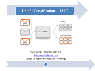
  • 1. Unit 3: Classification LH 7 Presented By : Tekendra Nath Yogi Tekendranath@gmail.com College Of Applied Business And Technology
  • 2. Contd… • Outline: – 3.1. Basics – 3.2. Decision Tree Classifier – 3.3. Rule Based Classifier – 3.4. Nearest Neighbor Classifier – 3.5. Bayesian Classifier – 3.6. Artificial Neural Network Classifier – 3.7. Issues : Over-fitting, Validation, Model Comparison 26/19/2019 By: Tekendra Nath Yogi
  • 3. June 19, 2019 By:Tekendra Nath Yogi 3 Introduction • Databases are rich with hidden information that can be used for intelligent decision making. • Classification and prediction are two forms of data analysis that can be used to extract models describing important data classes or to predict future data trends. Such analysis provide better understanding of the data at large. • classification predicts categorical (discrete, unordered) labels, prediction models continuous valued functions i.e., predicts unknown or missing values.
  • 4. June 19, 2019 By:Tekendra Nath Yogi 4 Contd… • When to use classification? – Following are the examples of cases where the data analysis task is Classification : • A bank loan officer wants to analyze the data in order to know which customer (loan applicant) are risky or which are safe. • A marketing manager at a company needs to analyze a customer with a given profile, who will buy a new computer. – In both of the above examples, a model or classifier is constructed to predict the categorical labels. These labels are risky or safe for loan application data and yes or no for marketing data.
  • 5. June 19, 2019 By:Tekendra Nath Yogi 5 Contd… • When to use Prediction? – Following are the examples of cases where the data analysis task is Prediction : • Suppose the marketing manager needs to predict how much a given customer will spend during a sale at his company. • In this example we are bothered to predict a numeric value. Therefore the data analysis task is an example of numeric prediction. • In this case, a model or a predictor will be constructed that predicts a continuous value.
  • 6. June 19, 2019 By:Tekendra Nath Yogi 6 How does classification work? • The Data Classification process includes two steps: – Building the Classifier or Model – Using Classifier for Classification
  • 7. June 19, 2019 By:Tekendra Nath Yogi 7 Contd… • Building the Classifier or Model: – Also known as model construction, training or learning phase – a classification algorithm builds the classifier (e.g., decision tree, if-then rules or mathematical formulae and etc) by analyzing or ―learning from‖ a training set made up of database tuples and their associated class labels. – Because the class label of each training tuple is provided, this step is also known as supervised learning – i.e., the learning of the classifier is ―supervised‖ in that it is told to which class each training tuple belongs.
  • 8. June 19, 2019 By:Tekendra Nath Yogi 8 Contd… • E.g.,
  • 9. June 19, 2019 By:Tekendra Nath Yogi 9 Contd… • Using Classifier for Classification: Before using the model, we first need to test its accuracy • Measuring model accuracy: – To measure the accuracy of a model we need test data (randomly selected from the general data set.) – Test data is similar in its structure to training data (labeled data) – How to test? – The known label of test sample is compared with the classified result from the model – Accuracy rate is the percentage of test set samples that are correctly classified by the model – Important: test data should be independent of training set, otherwise over- fitting will occur • Using the model: If the accuracy is acceptable, use the model to classify data tuples whose class labels are not known casestestofnumberTotal tionsclassificacorrectofNumber Accuracy
  • 10. June 19, 2019 By:Tekendra Nath Yogi 10 Contd… • E.g.,: • Here, Accuracy =3/4*100=75%
  • 11. June 19, 2019 By:Tekendra Nath Yogi 11 Contd… • Example to illustrate the steps of classification: – Model construction:
  • 12. June 19, 2019 By:Tekendra Nath Yogi 12 Contd… • Model Usage: Big spenders
  • 13. Classification by Decision Tree Induction • Decision tree induction is the learning of decision trees from class labeled training tuples • Decision tree is A flow-chart-like tree structure – Internal node denotes a test on an attribute – Branch represents an outcome of the test – Leaf nodes represent class labels or class distribution June 19, 2019 13By:Tekendra Nath Yogi
  • 14. June 19, 2019 By:Tekendra Nath Yogi 14 Contd… • How are decision trees used for classification? – The attributes of a tuple are tested against the decision tree – A path is traced from the root to a leaf node which holds the prediction for that tuple
  • 15. June 19, 2019 By:Tekendra Nath Yogi 15 Contd…
  • 16. Algorithm for Decision Tree Induction • Basic algorithm (a greedy algorithm) – At start, all the training examples are at the root – Samples are partitioned recursively based on selected attributes called the test attributes. – Test attributes are selected on the basis of a heuristic or statistical measure (e.g., information gain) • Conditions for stopping partitioning – All samples for a given node belong to the same class – There are no remaining attributes for further partitioning – majority voting is employed for classifying the leaf – There are no samples left June 19, 2019 16By:Tekendra Nath Yogi
  • 17. Algorithm for Decision Tree Induction (pseudocode) Algorithm GenDecTree(Sample S, Attlist A) 1. create a node N 2. If all samples are of the same class C then label N with C; terminate; 3. If A is empty then label N with the most common class C in S (majority voting); terminate; 4. Select aA, with the highest information gain; Label N with a; 5. For each value v of a: a. Grow a branch from N with condition a=v; b. Let Sv be the subset of samples in S with a=v; c. If Sv is empty then attach a leaf labeled with the most common class in S; d. Else attach the node generated by GenDecTree(Sv, A-a) June 19, 2019 17By:Tekendra Nath Yogi
  • 18. June 19, 2019 By:Tekendra Nath Yogi 18 Contd… • E.g.,
  • 19. June 19, 2019 By:Tekendra Nath Yogi 19 Contd…
  • 20. June 19, 2019 By:Tekendra Nath Yogi 20 Contd…
  • 21. June 19, 2019 By:Tekendra Nath Yogi 21 Contd…
  • 22. June 19, 2019 By:Tekendra Nath Yogi 22 Contd…
  • 23. June 19, 2019 By:Tekendra Nath Yogi 23 Contd…
  • 24. June 19, 2019 By:Tekendra Nath Yogi 24 Contd…
  • 25. June 19, 2019 By:Tekendra Nath Yogi 25 Attribute Selection Measures • An attribute selection measure is a heuristic for selecting the splitting criterion that ―best‖ separates a given data partition D • splitting rules – Provide ranking for each attribute describing the tuples – The attribute with highest score is chosen • Methods – Information gain – Gain ratio – Gini Index
  • 26. June 19, 2019 By:Tekendra Nath Yogi 26 Contd… • 1st approach: Information Gain Approach: – D: the current partition – N: represent the tuples of partition D – Select the attribute with the highest information gain – This attribute • minimizes the information needed to classify the tuples in the resulting partitions • reflects the least randomness or ―impurity‖ in these partitions – Information gain approach minimizes the expected number of tests needed to classify a given tuple and guarantees a simple tree
  • 27. June 19, 2019 By:Tekendra Nath Yogi 27 Contd… • Let pi be the probability that an arbitrary tuple in D (data set) belongs to class Ci, estimated by |Ci, D|/|D|  Expected information needed to classify a tuple in D:  Information needed (after using A to split D into v partitions) to classify D:  Information gained by branching on attribute A: )(log)( 2 1 i m i i ppDInfo   )( || || )( 1 j v j j A DI D D DInfo   (D)InfoInfo(D)Gain(A) A m: the number of classes
  • 28. June 19, 2019 By:Tekendra Nath Yogi 28 Contd… • Expected information needed to classify a tuple in D: )(log)( 2 1 i m i i ppDInfo  
  • 29. June 19, 2019 By:Tekendra Nath Yogi 29 Contd… • Information needed (after using A to split D into v partitions) to classify D: )( || || )( 1 j v j j A DI D D DInfo  
  • 30. June 19, 2019 By:Tekendra Nath Yogi 30 Contd… • Information gained by branching on attribute A: (D)InfoInfo(D)Gain(A) A
  • 31. Contd… income student credit_rating buys_computer high no fair no high no excellent no medium no fair no low yes fair yes medium yes excellent yes income student credit_rating buys_computer high no fair yes low yes excellent yes medium no excellent yes high yes fair yes income student credit_rating buys_computer medium no fair yes low yes fair yes low yes excellent no medium yes fair yes medium no excellent no age? Youth Middle aged Senior labeled yes • Because age has the highest information gain among the attributes, it is selected as the splitting attribute June 19, 2019 31By:Tekendra Nath Yogi
  • 32. Contd…. age? overcast student? credit rating? no yes fairexcellent youth senior no noyes yes yes Middle aged June 19, 2019 32By:Tekendra Nath Yogi Output: A Decision Tree for ―buys_computer Similarly,
  • 33. Contd… • Decision Tree Based Classification of Advantages: – Inexpensive to construct – Extremely fast at classifying unknown records – Easy to interpret for small-sized trees – Robust to noise (especially when methods to avoid over-fitting are employed) – Can easily handle redundant or irrelevant attributes (unless the attributes are interacting) June 19, 2019 33By:Tekendra Nath Yogi
  • 34. Contd… • Decision Tree Based Classification Disadvantages: – Space of possible decision trees is exponentially large. Greedy approaches are often unable to find the best tree. – Does not take into account interactions between attributes – Each decision boundary involves only a single attribute June 19, 2019 34By:Tekendra Nath Yogi
  • 35. June 19, 2019 By:Tekendra Nath Yogi 35 Naïve Bayes Classification • Bayesian classifiers are statistical classifiers. They can predict class membership probabilities, such as the probability that a given tuple belongs to a particular class. • i.e., For each new sample they provide a probability that the sample belongs to a class (for all classes). • Based on Bayes‘ Theorem
  • 36. June 19, 2019 By:Tekendra Nath Yogi 36 Contd… • Bayes‘ Theorem : – Given the training data set D and data sample to be classified X whose class label is unknown. – Let H be a hypothesis that X belongs to class C – Classification is to determine P(H|X), the probability that the hypothesis holds given the observed data sample X. – Predicts X belongs to Class Ci iff the probability P(Ci|X) is the highest among all the P(Ck|X) for all the k classes. – P(H), P(X|H), and P(X) can be estimated from the given data set. )( )()|()|( X XX P HPHPHP 
  • 37. June 19, 2019 By:Tekendra Nath Yogi 37 Contd… • The naïve Bayesian classifier, or simple Bayesian classifier, works as follows: 1. Let D be a training set of tuples and their associated class labels and X={x1, x2,…..xK} be a tuple that is to be classified based on D. i.e., unlabelled data whose class label is to be find. 2. In order to predict the class label of X, perform the following calculations for each class ci . a. Calculate Probability of each class ci as: P(Ci)=|Ci, D|/|D|, where |Ci, D| is the number of training tuples of class Ci in D.
  • 38. June 19, 2019 By:Tekendra Nath Yogi 38 Contd… b) For each value of attributes in X calculate P(xk|Ci)As: c) Calculate the Probalility of a tuple X conditioned on class Ci as: d) Calculate the probalility of class ci , conditioned on X as: P(Ci|X)= P(X|Ci)*P(Ci). 3. predict the class label of X as: The predicted class label of X is the class Ci for which P(X|Ci)*P(Ci) is the maximum. )|(...)|()|( 1 )|()|( 21 CixPCixPCixP n k CixPCiP nk   X DinCiclassoftuplesofnumberthe|,DCi,| AkattributeforxkvaluethehavingDinCiclassoftuples# Ci)|P(xk 
  • 39. June 19, 2019 By:Tekendra Nath Yogi 39 Contd… • Example: study the training data given below and construct a Naïve Bayes classifier and then classify the given sample. • Training set: • classify a new sample X = (age <= 30 , income = medium, student = yes, credit_rating = fair) age income studentcredit_ratingbuys_computer <=30 high no fair no <=30 high no excellent no 31…40 high no fair yes >40 medium no fair yes >40 low yes fair yes >40 low yes excellent no 31…40 low yes excellent yes <=30 medium no fair no <=30 low yes fair yes >40 medium yes fair yes <=30 medium yes excellent yes 31…40 medium no excellent yes 31…40 high yes fair yes >40 medium no excellent no
  • 40. June 19, 2019 By:Tekendra Nath Yogi 40 Contd… • Solution: In the given training data set two classes yes and no are present. – Let, C1:buys_computer = ‗yes‘ and C2:buys_computer = ‗no‘ • Calculate Probability of each class ci as: P(Ci)=|Ci, D|/|D|, where |Ci, D| is the number of training tuples of class Ci in D. – P(buys_computer = ―yes‖) = 9/14 = 0.643 – P(buys_computer = ―no‖) = 5/14= 0.357 age income studentcredit_ratingbuys_compute <=30 high no fair no <=30 high no excellent no 31…40 high no fair yes >40 medium no fair yes >40 low yes fair yes >40 low yes excellent no 31…40 low yes excellent yes <=30 medium no fair no <=30 low yes fair yes >40 medium yes fair yes <=30 medium yes excellent yes 31…40 medium no excellent yes 31…40 high yes fair yes >40 medium no excellent no
  • 41. June 19, 2019 By:Tekendra Nath Yogi 41 Contd… • Compute P(XK|Ci) for each class: P(age = ―<=30‖ | buys_computer = ―yes‖) = 2/9 = 0.222 P(age = ―<= 30‖ | buys_computer = ―no‖) = 3/5 = 0.6 P(income = ―medium‖ | buys_computer = ―yes‖) = 4/9 = 0.444 P(income = ―medium‖ | buys_computer = ―no‖) = 2/5 = 0.4 P(student = ―yes‖ | buys_computer = ―yes) = 6/9 = 0.667 P(student = ―yes‖ | buys_computer = ―no‖) = 1/5 = 0.2 P(credit_rating = ―fair‖ | buys_computer = ―yes‖) = 6/9 = 0.667 P(credit_rating = ―fair‖ | buys_computer = ―no‖) = 2/5 = 0.4
  • 42. June 19, 2019 By:Tekendra Nath Yogi 42 Contd… • Compute P(X|Ci) for each class: – P(X|buys_computer = ―yes‖) = 0.222 x 0.444 x 0.667 x 0.667 = 0.044 – P(X|buys_computer = ―no‖) = 0.6 x 0.4 x 0.2 x 0.4 = 0.019 • Calculate the probalility of class ci , conditioned on X as: P(Ci|X)=P(X|Ci)*P(Ci) – P(buys_computer = ―yes‖ | X ) =P(X|buys_computer = ―yes‖) * P(buys_computer = ―yes‖) = 0.028 (maximum). – P(buys_computer = ―no‖ |X) = P(X|buys_computer = ―no‖) * P(buys_computer = ―no‖) = 0.007 • Therefore, X belongs to class (“buys_computer = yes”)
  • 43. 43 Contd… • Avoiding the 0-Probability Problem: – Naïve Bayesian prediction requires each conditional prob. be non-zero. Otherwise, the predicted prob. will be zero – Ex. Suppose a dataset with 1000 tuples, income=low (0), income= medium (990), and income = high (10), – Use Laplacian correction • Adding 1 to each case Prob(income = low) = 1/1003 Prob(income = medium) = 991/1003 Prob(income = high) = 11/1003 • The ―corrected‖ prob. estimates are close to their ―uncorrected‖ counterparts    n k CixkPCiXP 1 )|()|( June 19, 2019 By:Tekendra Nath Yogi
  • 44. 44 Contd… • Advantages – Easy to implement – Good results obtained in most of the cases • Disadvantages – Assumption: class conditional independence, therefore loss of accuracy – Practically, dependencies exist among variables • E.g., hospitals: patients: Profile: age, family history, etc. Symptoms: fever, cough etc., Disease: lung cancer, diabetes, etc. • Dependencies among these cannot be modeled by Naïve Bayesian Classifier June 19, 2019 By:Tekendra Nath Yogi
  • 45. June 19, 2019 By:Tekendra Nath Yogi 45 Contd… • Example: study the training data given below and construct a Naïve Bayes classifier and then classify the given sample. • Training set: • classify a new sample X:< outlook = sunny, temperature = cool, humidity = high, windy = false> Outlook Temperature Humidity Windy Class sunny hot high false N sunny hot high true N overcast hot high false P rain mild high false P rain cool normal false P rain cool normal true N overcast cool normal true P sunny mild high false N sunny cool normal false P rain mild normal false P sunny mild normal true P overcast mild high true P overcast hot normal false P rain mild high true N play tennis?
  • 46. June 19, 2019 By:Tekendra Nath Yogi 46 Contd… • Solution: Outlook Temperature Humidity Windy Class sunny hot high false N sunny hot high true N rain cool normal true N sunny mild high false N rain mild high true N Outlook Temperature Humidity Windy Class overcast hot high false P rain mild high false P rain cool normal false P overcast cool normal true P sunny cool normal false P rain mild normal false P sunny mild normal true P overcast mild high true P overcast hot normal false P 9 5
  • 47. June 19, 2019 By:Tekendra Nath Yogi 47 Contd… • Given the training set, we compute the probabilities: • We also have the probabilities – P = 9/14 – N = 5/14 O utlook P N Hum idity P N sunny 2/9 3/5 high 3/9 4/5 overcast 4/9 0 norm al 6/9 1/5 rain 3/9 2/5 Tem preature W indy hot 2/9 2/5 true 3/9 3/5 m ild 4/9 2/5 false 6/9 2/5 cool 3/9 1/5
  • 48. June 19, 2019 By:Tekendra Nath Yogi 48 Contd… • To classify a new sample X: < outlook = sunny, temperature = cool, humidity = high, windy = false> • Prob(P|X) = Prob(P)*Prob(sunny|P)*Prob(cool|P)* Prob(high|P)*Prob(false|P) = 9/14*2/9*3/9*3/9*6/9 = 0.01 • Prob(N|X) =Prob(N)*Prob(sunny|N)*Prob(cool|N)*Prob(high|N)*Prob(false|N) = 5/14*3/5*1/5*4/5*2/5 = 0.013 • Therefore X takes class label N
  • 49. Artificial Neural Network • A neural network is composed of number of nodes or units , connected by links. Each link has a numeric weight associated with it. • Actually artificial neural networks are programs design to solve any problem by trying to mimic the structure and the function of our nervous system. 496/19/2019 Presented By: Tekendra Nath Yogi 2 1 3 4 5 6 Input Layer Hidden Layer Output Layer
  • 50. Artificial neural network model: • Input to the network are represented by mathematical symbol xn. • Each of these inputs are multiplied by a connection weight, wn • These products are simply summed, fed through the transfer function f() to generate result and output 50 nnxwxwxwsum  ......2211 6/19/2019 Presented By: Tekendra Nath Yogi
  • 51. Back propagation algorithm • Back propagation is a neural network learning algorithm. Learns by adjusting the weight so as to be able to predict the correct class label of the input. Input: D training data set and their associated class label l= learning rate(normally 0.0-1.0) Output: a trained neural network. Method: Step1: initialize all weights and bias in network. Step2: while termination condition is not satisfied . For each training tuple x in D 516/19/2019 Presented By: Tekendra Nath Yogi
  • 52. 2.1 calculate output: For input layer For hidden layer and output layer 52 jj IO  e j j jkjk I k j O WOI      1 1 *  Contd… 6/19/2019 Presented By: Tekendra Nath Yogi
  • 53. 2.2 Calculate error: For output layer: For hidden layer: 2.3 Update weight 2.4 Update bias 53 ))(1( jjjjj OOOerr   )*()1(  k jkkjjj WerrOOerr jiijij errOloldWnewW **)()(  jjj errl * Contd… 6/19/2019 Presented By: Tekendra Nath Yogi
  • 54. 6/19/2019 Presented By: Tekendra Nath Yogi 54 Contd… • Example: Sample calculations for learning by the back-propagation algorithm. • Figure above shows a multilayer feed-forward neural network. Let the learning rate be 0.9. The initial weight and bias values of the network are given in Table below, along with the first training tuple, X = (1, 0, 1), whose class label is 1. 1
  • 55. 6/19/2019 Presented By: Tekendra Nath Yogi 55 Contd… • Step1: Initialization – Let initial input weight and bias values are: – Initial input: – Bias values: – Initial weight: X1 X2 X3 1 0 1 -0.4 0.2 0.1 4 W14 W15 W24 W25 W34 W35 W46 W56 0.2 -0.3 0.4 0.1 -0.5 0.2 -0.3 -0.2 5 6
  • 56. 6/19/2019 Presented By: Tekendra Nath Yogi 56 Contd… • 2. Termination condition: Weight of two successive iteration are nearly equal or user defined number of iterations are reached. • 2.1For each training tuple X in D, calculate the output for each input layer: – For input layer: • O1=I1=1 • O2=I2=0 • O3=I3=1 jj IO 
  • 57. 6/19/2019 Presented By: Tekendra Nath Yogi 57 Contd… • For hidden layer and output layer: 1. 2. 332.0 )7182.2(1 1 1 1 1 1 0.7- (-0.5)*10.4*00.2*1 4W34*O3W24*O2W14*O1 )7.0()7.0(4 4 4             ee I O I  525.0 )7182.2(1 1 1 1 1 1 0.1 0.2*10.1*0(-0.3)*1 5W35*O3W25*O2W15*O1 )1.0()1.0(5 5 5            ee I O I 
  • 58. 6/19/2019 Presented By: Tekendra Nath Yogi 58 Contd… 3. 474.0 )7182.2(1 1 1 1 1 1 0.105- 0.1*1(-0.2)*0.5250.3)(*332.0 5W56*O5W46*O4 )105.0()105.0(6 6 6              ee I O I 
  • 59. 6/19/2019 Presented By: Tekendra Nath Yogi 59 Contd… • Calculation of error at each node: • For output layer: • For Hidden layer: 1311.0)474.01)(474.01(474.0 ))(1( ))(1( 66666    OOOerr OOOerr jjjjj   0087.0 ))3.0(*1311.0)(332.01(332.0 )*)(1( )*)(1( 0065.0 ))2.0(*1311.0)(525.01(525.0 )*)(1( )*)(1( )*()1( 46644 56655           WerrOO WerrOOerr WerrOO WerrOOerr WerrOOerr • jkkjjj • jkkjjj jkkjjj k
  • 60. 6/19/2019 Presented By: Tekendra Nath Yogi 60 Contd… • Update the weight: 1. 2. 3. jiijij errOloldWnewW **)()(  26.0 332.0*1311.0*9.03.0 **)()( 644646    errOloldWnewW 138.0 525.0*1311.0*9.02.0 **)()( 655656    errOloldWnewW 192.0 1*0087.0*9.02.0 **)()( 411414    errOloldWnewW
  • 61. 6/19/2019 Presented By: Tekendra Nath Yogi 61 Contd… 4. 5. 6. 4.0 0*0087.0(*9.04.0 **)()( 422424    errOloldWnewW 306.0 1*)0065.0(*9.03.0 **)()( 511515    errOloldWnewW 508.0 1*0087.0(*9.05.0 **)()( 433434    errOloldWnewW
  • 62. 6/19/2019 Presented By: Tekendra Nath Yogi 62 Contd… 7. 8. 194.0 1*)0065.0(*9.02.0 **)()( 533535    errOloldWnewW 1.0 0*)0065.0(*9.01.0 **)()( 522525    errOloldWnewW
  • 63. 6/19/2019 Presented By: Tekendra Nath Yogi 63 Contd… • Update the Bias value: 1. 2. 3. And so on until convergence! jjj errl * 218.0 1311.0*9.01.0 * 6)(66    errlold 195.0 )0065.0(*9.02.0 * 5)(55    errlold 408.0 )0087.0(*9.0)4.0( * 4)(46    errlold
  • 64. Rule Based Classifier • In Rule based classifiers learned model is represented as a set of If-Then rules. • A rule-based classifier uses a set of IF-THEN rules for classification. • An IF-THEN rule is an expression of the form – IF condition THEN conclusion. – An example is : IF(Give Birth = no)  (Can Fly = yes) THEN Birds • The ―IF‖ part (or left side) of a rule is known as the rule antecedent or precondition. • The ―THEN‖ part (or right side) is the rule consequent. In the rule antecedent, the condition consists of one or more attribute tests (e.g., (Give Birth = no)  (Can Fly = yes)) That are logically ANDed. The rule‘s consequent contains a class prediction. May 20, 2018 64By: Tekendra Nath Yogi
  • 65. Contd.. • Rule-based Classifier (Example) May 20, 2018 65By: Tekendra Nath Yogi Name Blood Type Give Birth Can Fly Live in Water Class human warm yes no no mammals python cold no no no reptiles salmon cold no no yes fishes whale warm yes no yes mammals frog cold no no sometimes amphibians komodo cold no no no reptiles bat warm yes yes no mammals pigeon warm no yes no birds cat warm yes no no mammals leopard shark cold yes no yes fishes turtle cold no no sometimes reptiles penguin warm no no sometimes birds porcupine warm yes no no mammals eel cold no no yes fishes salamander cold no no sometimes amphibians gila monster cold no no no reptiles platypus warm no no no mammals owl warm no yes no birds dolphin warm yes no yes mammals eagle warm no yes no birds R1: (Give Birth = no)  (Can Fly = yes)  Birds R2: (Give Birth = no)  (Live in Water = yes)  Fishes R3: (Give Birth = yes)  (Blood Type = warm)  Mammals R4: (Give Birth = no)  (Can Fly = no)  Reptiles R5: (Live in Water = sometimes)  Amphibians
  • 66. How does Rule-based Classifier Work? R1: (Give Birth = no)  (Can Fly = yes)  Birds R2: (Give Birth = no)  (Live in Water = yes)  Fishes R3: (Give Birth = yes)  (Blood Type = warm)  Mammals R4: (Give Birth = no)  (Can Fly = no)  Reptiles R5: (Live in Water = sometimes)  Amphibians A lemur triggers rule R3, so it is classified as a mammal A turtle triggers both R4 and R5 A dogfish shark triggers none of the rules Name Blood Type Give Birth Can Fly Live in Water Class lemur warm yes no no ? turtle cold no no sometimes ? dogfish shark cold yes no yes ? May 20, 2018 66By: Tekendra Nath Yogi
  • 67. May 20, 2018 By: Tekendra Nath Yogi 67 age? student? credit rating? <=30 >40 no yes yes yes 31..40 fairexcellentyesno • Example: Rule extraction from our buys_computer decision-tree IF age = young AND student = no THEN buys_computer = no IF age = young AND student = yes THEN buys_computer = yes IF age = mid-age THEN buys_computer = yes IF age = old AND credit_rating = excellent THEN buys_computer = yes IF age = young AND credit_rating = fair THEN buys_computer = no Rule Extraction from a Decision Tree  Rules are easier to understand than large trees  One rule is created for each path from the root to a leaf  Each attribute-value pair along a path forms a conjunction: the leaf holds the class prediction
  • 68. Rule Coverage and Accuracy • A Rule R can be assessed by its coverage and accuracy • Coverage of a rule: – Fraction of records that satisfy the antecedent of a rule • Accuracy of a rule: – Fraction of records that satisfy the antecedent that also satisfy the consequent of a rule Tid Refund Marital Status Taxable Income Class 1 Yes Single 125K No 2 No Married 100K No 3 No Single 70K No 4 Yes Married 120K No 5 No Divorced 95K Yes 6 No Married 60K No 7 Yes Divorced 220K No 8 No Single 85K Yes 9 No Married 75K No 10 No Single 90K Yes 10 (Status=Single)  No Coverage = 40%, Accuracy = 50% May 20, 2018 68By: Tekendra Nath Yogi
  • 69. Contd.. • Advantages of Rule-Based Classifiers: – As highly expressive as decision trees – Easy to interpret – Easy to generate – Can classify new instances rapidly – Performance comparable to decision trees May 20, 2018 69By: Tekendra Nath Yogi
  • 70. K-Nearest Neighbor (KNN) Classifier • KNN is a non-parametric, lazy learning algorithm. • non-parametric: – means that it does not make any assumptions on the underlying data distribution. – Therefore, KNN used when there is little or no prior knowledge about the data distribution. • Lazy: – means that it does not have explicit training phase or it is very minimal. June 19, 2019 70By: Tekendra Nath Yogi
  • 71. Contd…. • KNN stores the entire training dataset which it uses as its representation. i.e., KNN does not learn any model. • A positive integer k ( number of nearest neighbors) is specified, along with a new sample X. • KNN makes predictions just-in-time by calculating the similarity between an input sample and each training instance. • We select the k entries in our training data set which are closest to the new sample • We find the most common classification of these entries ( majority voting). • This is the classification we give to the new sample June 19, 2019 71By: Tekendra Nath Yogi
  • 72. Contd…. June 19, 2019 72By: Tekendra Nath Yogi
  • 73. Contd…. • KNN Algorithm: – Read the training data D, data sample to be classified X and the value of k ( number of nearest neighbors) – For getting the predicted class of X, iterate from 1 to total number of training data points • Calculate the Euclidean distance between X and each row of training data. • Sort the calculated distances in ascending order based on distance values • Get top k rows from the sorted array • Get the most frequent class of these rows • Return the predicted class June 19, 2019 73By: Tekendra Nath Yogi
  • 74. Contd…. • According to the Euclidean distance formula, the distance between two points in the plane with coordinates (x, y) and (a, b) is given by June 19, 2019 74By: Tekendra Nath Yogi dist((x, y), (a, b)) = √(x - a)² + (y - b)² dist((2, -1), (-2, 2)) = √(2 - (-2))² + ((-1) - 2)² = √(2 + 2)² + (-1 - 2)² = √(4)² + (-3)² = √16 + 9 = √25 = 5. • As an example, the (Euclidean) distance between points (2, -1) and (-2, 2) is found to be
  • 75. Contd…. • Example1: Apply KNN algorithm and predict the class for X= (3, 7) on the basis of following training data set with K=3. June 19, 2019 75By: Tekendra Nath Yogi p q Class label 7 7 False 7 4 False 3 4 True 1 4 True
  • 76. Contd…. • Solution: – Given, k= 3 and new data same to be classified X= (3, 7) – Now, computing the Euclidean distance between X and each tuples in the training set: June 19, 2019 76By: Tekendra Nath Yogi d1((3, 7), (7, 7)) = √(3 - 7)² + (7 - 7)² = √(4)² + (0)² =4 d1((3, 7), (7, 4)) = √(3 - 7)² + (7 - 4)² = √(4)² + (3)² =5 d1((3, 7), (3, 4)) = √(3 - 3)² + (7 - 4)² = √(0)² + (3)² =3 d1((3, 7), (1, 4)) = √(3 - 1)² + (7 - 4)² = √(2)² + (3)² =3.6
  • 77. Contd…. • Now, sorting the data samples in a training set in ascending order of their distance from the new sample to be classified . • Now , deciding the category of X based on the majority classes in top K=3 samples as: • Here, in top 3 data True class has majority so the data sample X= (3, 7) belong to the class True. June 19, 2019 77By: Tekendra Nath Yogi p q class Distance (X, D) 3 4 True 3 1 4 True 3.6 7 7 False 4 7 4 False 5 p q class Distance (X, D) 3 4 True 3 1 4 True 3.6 7 7 False 4 7 4 False 5
  • 78. Contd…. • Example2: Apply KNN algorithm and predict the class for X= (6, 4) on the basis of following training data set with K=3. June 19, 2019 78By: Tekendra Nath Yogi p q Category 8 5 bad 3 7 good 3 6 good 7 3 bad
  • 79. Some pros and cons of KNN • Pros: – No assumptions about data — useful, for example, for nonlinear data – Simple algorithm — to explain and understand – High accuracy (relatively) — it is pretty high but not competitive in comparison to better supervised learning models – Versatile — useful for classification or regression • Cons: – Computationally expensive — because the algorithm Stores all (or almost all) of the training data – High memory requirement – Prediction stage might be slow June 19, 2019 79By: Tekendra Nath Yogi
  • 80. June 20, 2019 Data Mining: Concepts and Techniques 80 Lazy vs. Eager Learning • Lazy vs. eager learning – Lazy learning: Simply stores training data (or only minor processing) and waits until it is given a test tuple – Eager learning: Given training set, constructs a classification model before receiving new data to classify • Lazy: less time in training but more time in predicting • Accuracy – Lazy method effectively uses a richer hypothesis space since it uses many local linear functions to form its implicit global approximation to the target function – Eager: must commit to a single hypothesis that covers the entire instance space
  • 81. Issues regarding classification and prediction (2): Evaluating Classification Methods • accuracy • Speed – time to construct the model – time to use the model • Robustness – handling noise and missing values • Scalability – efficiency in disk-resident databases • Interpretability: – understanding and insight provided by the model • Goodness of rules (quality) – decision tree size – compactness of classification rules May 20, 2018 81By: Tekendra Nath Yogi
  • 82. CS583, Bing Liu, UIC 82 Evaluation methods • Holdout Method: The available data set D is divided into two disjoint subsets, – the training set Dtrain (for learning a model) – the test set Dtest (for testing the model) • Important: training set should not be used in testing and the test set should not be used in learning. – Unseen test set provides a unbiased estimate of accuracy. • The test set is also called the holdout set. (the examples in the original data set D are all labeled with classes.) • This method is mainly used when the data set D is large.
  • 83. CS583, Bing Liu, UIC 83 Evaluation methods (cont…) • k-fold cross-validation: The available data is partitioned into k equal-size disjoint subsets. • Use each subset as the test set and combine the rest n-1 subsets as the training set to learn a classifier. • The procedure is run k times, which give k accuracies. • The final estimated accuracy of learning is the average of the k accuracies. • 10-fold and 5-fold cross-validations are commonly used. • This method is used when the available data is not large.
  • 84. CS583, Bing Liu, UIC 84 Evaluation methods (cont…) • Leave-one-out cross-validation: This method is used when the data set is very small. • It is a special case of cross-validation • Each fold of the cross validation has only a single test example and all the rest of the data is used in training. • If the original data has m examples, this is m-fold cross- validation
  • 85. CS583, Bing Liu, UIC 85 Evaluation methods (cont…) • Validation set: the available data is divided into three subsets, – a training set, – a test set and – a validation set • A validation set is used frequently for estimating parameters in learning algorithms. • In such cases, the values that give the best accuracy on the validation set are used as the final parameter values. • Cross-validation can be used for parameter estimating as well.
  • 86. Home Work • What is supervised classification? In what situations can this technique be useful? • What is classification? Briefly outline the major steps of decision tree classification. • Why naïve Bayesian classification called naïve? Briefly outline the major idea of naïve Bayesian classification. • Compare the advantages and disadvantages of eager classification versus lazy classification. • Write an algorithm for k-nearest- neighbor classification given k, the nearest number of neighbors, and n, the number of attributes describing each tuple. May 20, 2018 By: Tekendra Nath Yogi 86
  • 87. Thank You ! 87By: Tekendra Nath Yogi6/19/2019