1. MS Excel 2010 Formulas
AutoSum and Excel Equations
One of the most powerful features of Excel is its ability to perform basic math functions on
data. Excel can add, subtract, multiply, divide, find the average, and perform general
counting functions on the numerical data that you enter. To enable this feature, highlight all
of the cells in a column, plus one additional empty cell in which to display the result.
Select the AutoSum icon from the ribbon menu:
If you click directly on the ∑, Excel will automatically add up the numbers
you have selected. If you click on the little dropdown arrow next to it
(▼), you will get the full choice of mathematical functions.
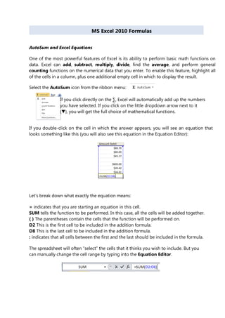
If you double-click on the cell in which the answer appears, you will see an equation that
looks something like this (you will also see this equation in the Equation Editor):
Let’s break down what exactly the equation means:
= indicates that you are starting an equation in this cell.
SUM tells the function to be performed. In this case, all the cells will be added together.
( ) The parentheses contain the cells that the function will be performed on.
D2 This is the first cell to be included in the addition formula.
D8 This is the last cell to be included in the addition formula.
: indicates that all cells between the first and the last should be included in the formula.
The spreadsheet will often “select” the cells that it thinks you wish to include. But you
can manually change the cell range by typing into the Equation Editor.

2. When you are ready to execute the formula, just press the “Enter” key.
Other mathematical functions you can perform from the AutoSum button include:
Average – This function will calculate the average of the selected cells. Count
Numbers – This function simply counts the number of cells selected. Max –
This function will return the highest value of the selected cells.
Min – This function will return the lowest value of the selected cells.
*Remember* Excel equations are similar to programming languages, so have some
patience and if at first you don’t succeed, try again. Even Excel professionals create
incorrect formulas on their first try.
Once you get an equation to work, you will technically be a computer programmer!

3. Conditional & Logical Functions
Excel has a number of logical functions which allow you to set various “conditions”
and have data respond to them. For example, you may only want a certain calculation
performed or piece of text displayed if certain conditions are met. The functions used
to produce this type of analysis are found in the Insert, Function menu, under the
heading LOGICAL.
If Statements
The IF function is used to analyse data, test whether or not it meets certain
conditions and then act upon its decision. The formula can be entered either by
typing it or by using the Function Library on the formula’s ribbon, the section that
deals with logical functions Typically, the IF statement is accompanied by three
arguments enclosed in one set of parentheses; the condition to be met
(logical_test); the action to be performed if that condition is true (value_if_true); the
action to be performed if false (value_if_false). Each of these is separated by a
comma, as shown;

4. =IF ( logical_test, value_if_true, value_if_false) To view IF function syntax:
Mouse
1. Click the drop down arrow next to the LOGICAL button in the FUNCTION LIBARY
Groupon the
FORMULAS
Ribbon;
2. A dialog box will appear
3. The three arguments can be seen within the box

5. Logical Test
This part of the IF statement is the “condition”, or test. You may want to test to see if
a cell is a certain value, or to compare two cells. In these cases, symbols called
LOGICAL OPERATORS are useful;
> Greater
than
< Less
than
> = Greater than or equal to
< = Less than or equal to
= Equal
to
<> Not equal
to
Therefore, a typical logical test might be B1>B2, testing whether or not the value
contained in cell B1 of the spreadsheet is greater than the value in cell B2. Names
can also be included in the logical test, so if cells B1 and B2 were respectively named
SALES and TARGET, the logical test would read SALES>TARGET. Another type of
logical test could include text strings. If you want to check a cell to see if it contains
text, that text string must be included in quotation marks. For example, cell C5
could be tested for the word YES as follows; C5=”YES”.
It should be noted that Excel’s logic is, at times, brutally precise. In the above
example, the logical test is that sales should be greater than target. If sales are equal
to target, the IF statement will return the false value. To make the logical test more
flexible, it would be advisable to use the operator >= to indicate “meeting or
exceeding”.
Value If True / False
Provided that you remember that TRUE value always precedes FALSE value, these
two values can be almost anything. If desired, a simple number could be returned,
a calculation performed, or even a piece of text entered. Also, the type of data
entered can vary depending on whether it is a true or false result. You may want a
calculation if the logical test is true, but a message displayed if false. (Remember that
text to be included in functions should be enclosed in quotes).

6. Taking the same logical test mentioned above, if the sales figure meets or exceeds the
target, a BONUS is calculated (e.g.2% of sales). If not, no bonus is calculated so a
value of zero is returned. The IF statement in column D of the example reads as
follows;
=IF(B2>=C2,B2*2%,0)
You may, alternatively, want to see a message saying “NO BONUS”. In this case, the true
value will remain the same and the false value will be the text string “NO BONUS”;
= IF(B2>=C2,B2*2%,”NO BONUS”)
A particularly common use of IF statements is to produce “ratings” or “comments” on
figures in a spreadsheet. For this, both the true and false values are text strings. For
example, if a sales figure exceeds a certain amount, a rating of “GOOD” is returned,
otherwise the rating is “POOR”;
=IF(B2>1000,”GOOD”,”POOR”)
Nested If
When you need to have more than one condition and more than two possible
outcomes, a NESTED IF is required. This is based on the same principle as a normal IF
statement, but involves “nesting” a secondary formula inside the main one. The

7. secondary IF forms the FALSE part of the main statement, as follows;
=IF(1st logic test , 1st true value , IF(2nd logic test , 2nd true value , false value))
Only if both logic tests are found to be false will the false value be returned. Notice that
there are two sets of parentheses, as there are two separate IF statements. This process
can be enlarged to include more conditions and more eventualities - up to seven IF’s
can be nested within the main statement. However, care must be taken to ensure that
the correct number of parentheses are added.
In the example, sales staff could now receive one of three possible ratings;
=IF(B2>1000,”GOOD”,IF(B2<600,”POOR”,”AVERAGE”))
To make the above IF statement more flexible, the logical tests could be amended to
measure sales against cell references instead of figures. In the example, column E has
been used to hold the upper and lower sales thresholds.
=IF(B2>$E$2,”GOOD”,IF(B2<$E$3,”POOR”,”AVERAGE”))
(If the IF statement is to be copied later, this cell reference should be
absolute).
N.B. The depth of nested IF functions has been increased to 64 as previous versions of
excel only nested 7 deep