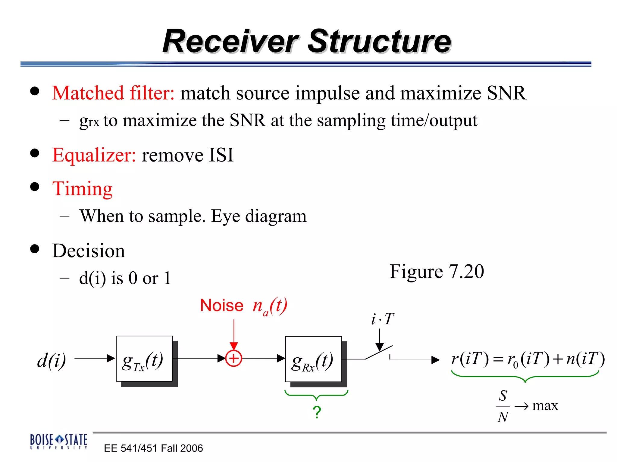
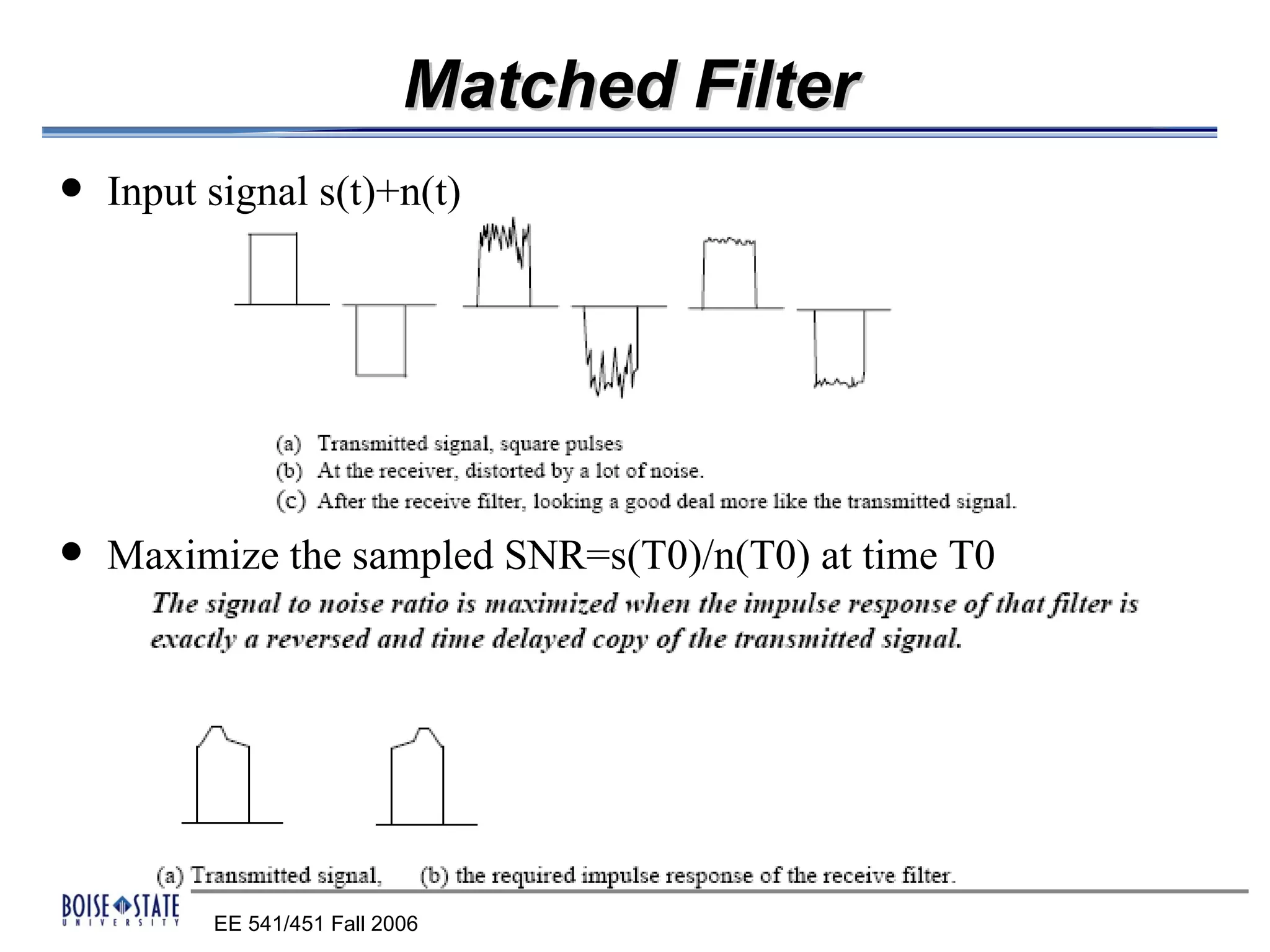
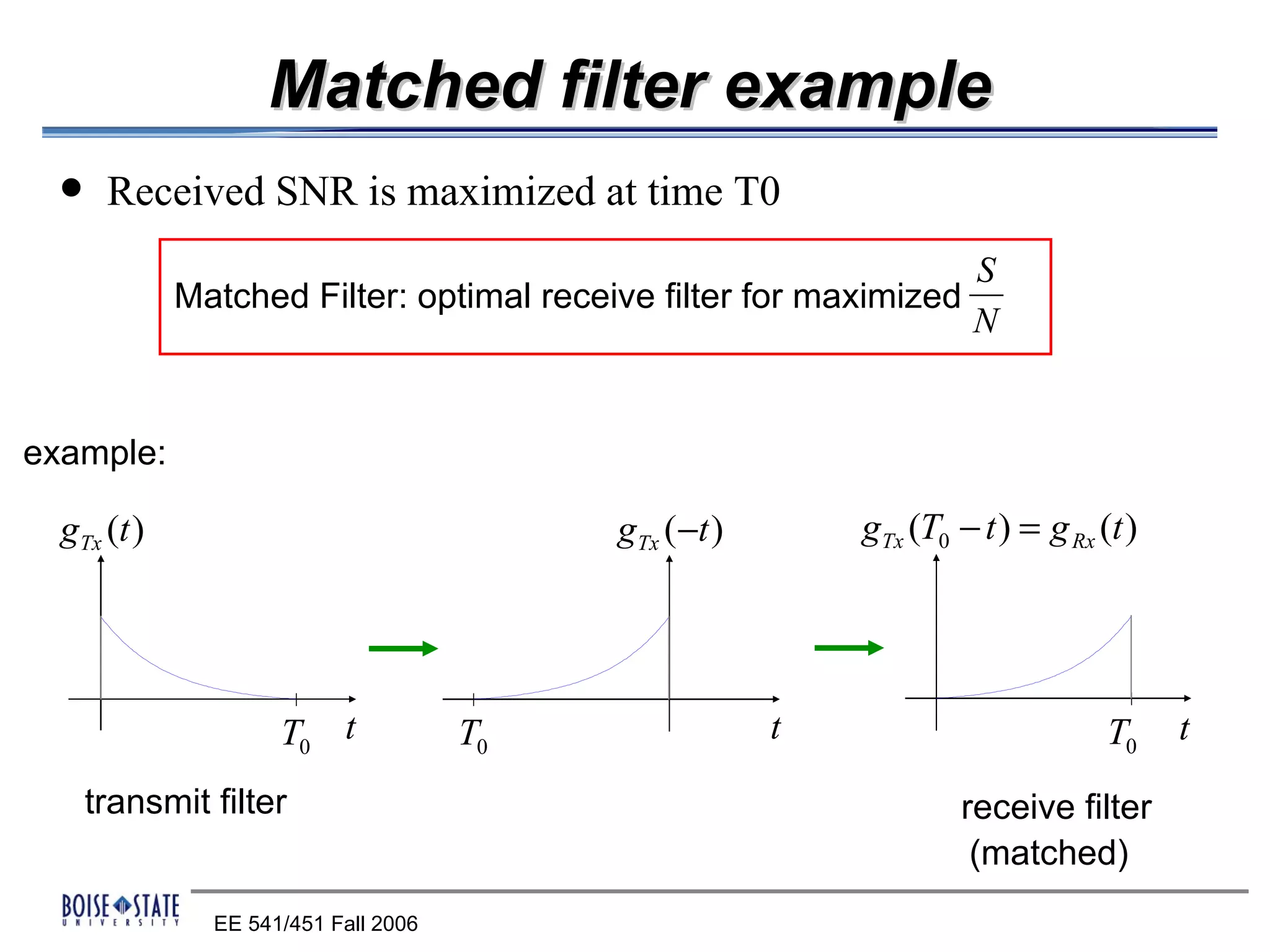
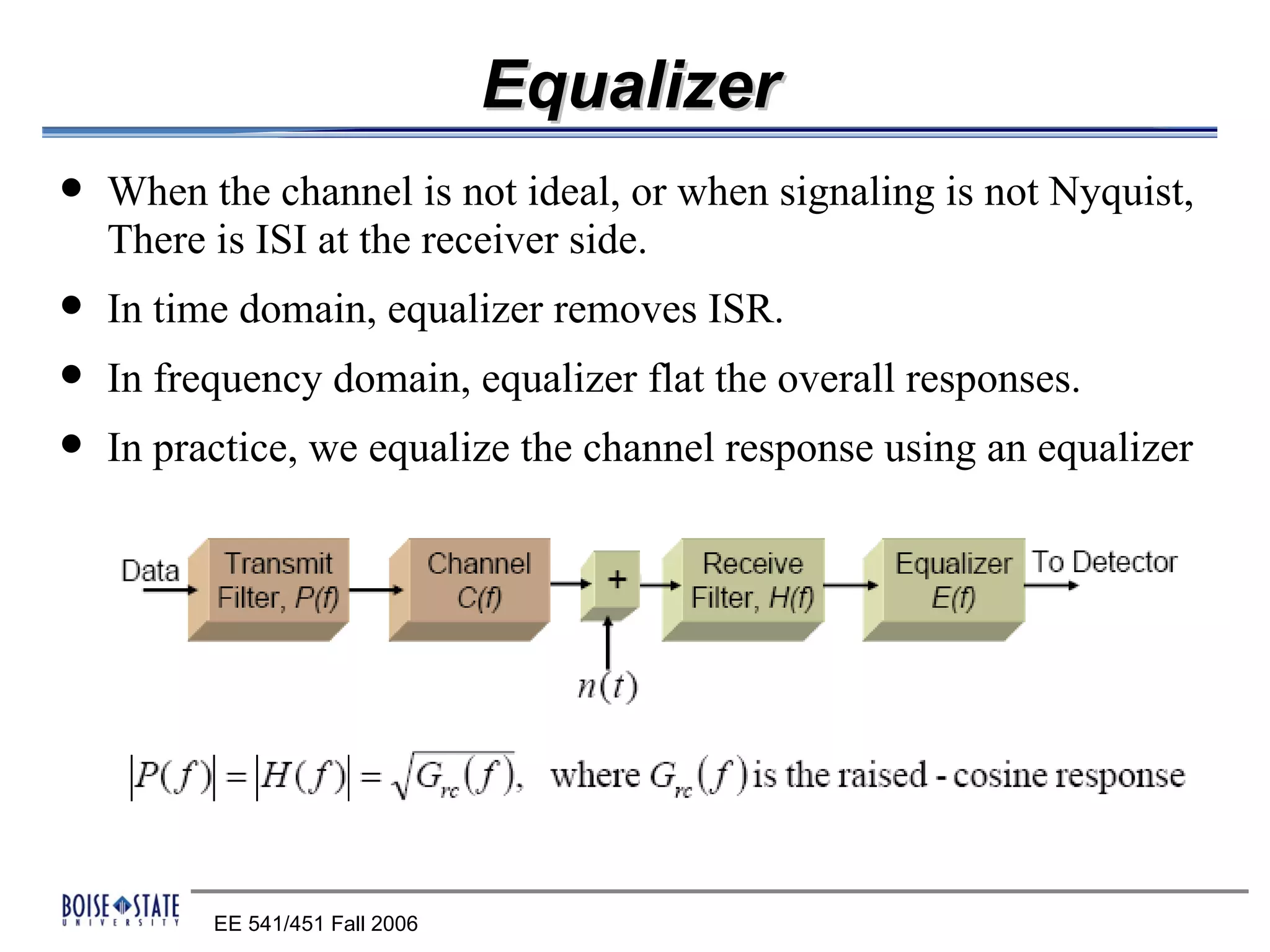
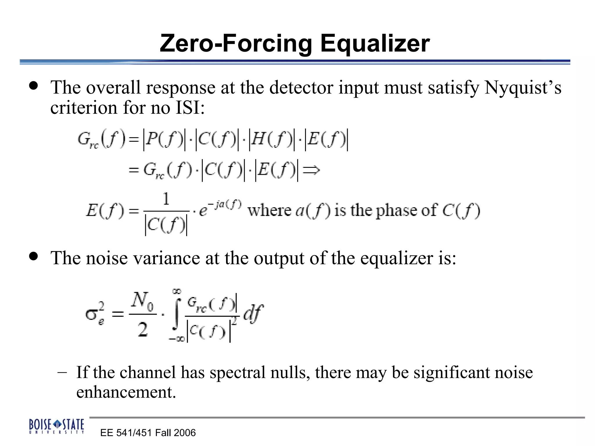
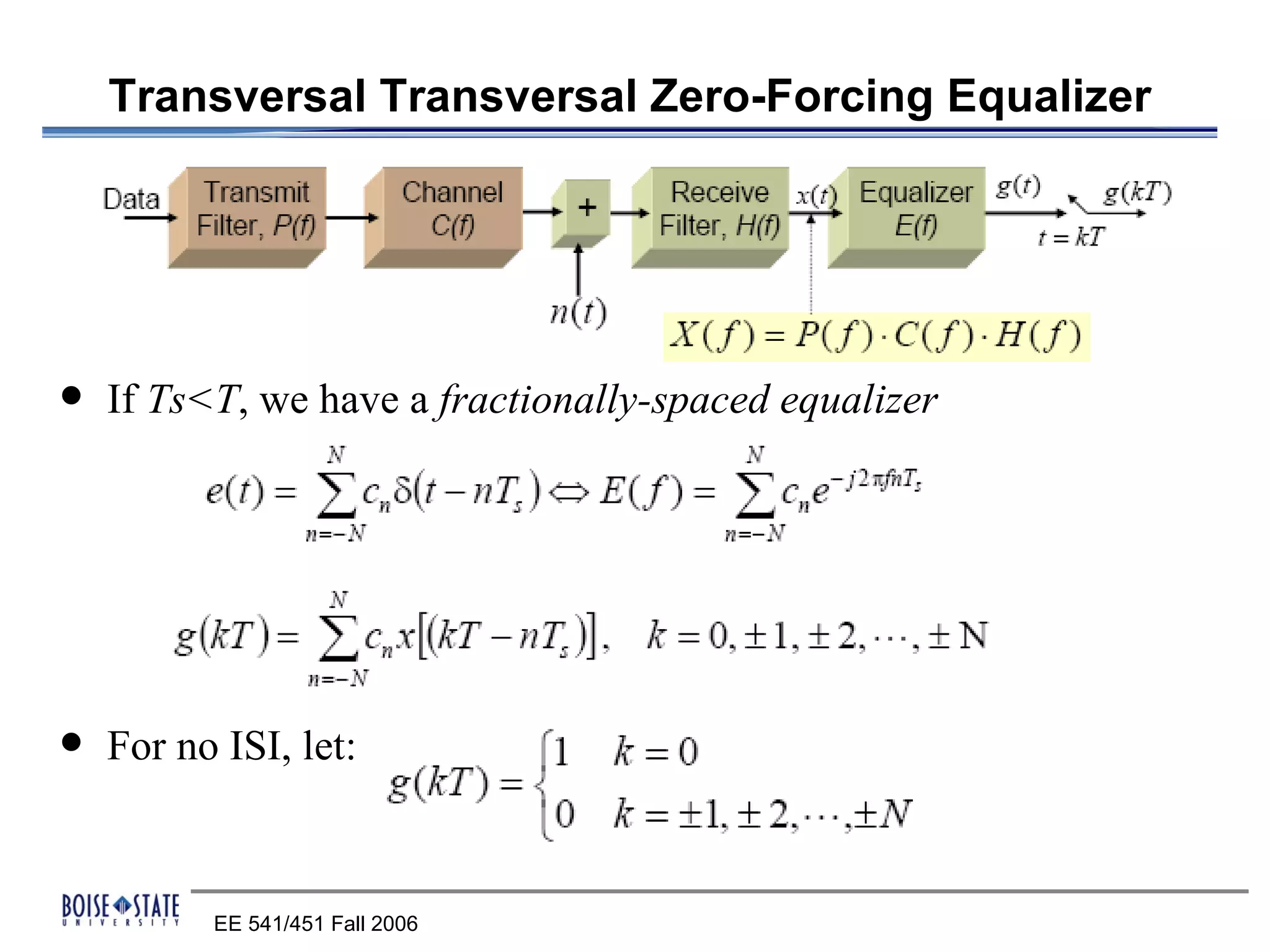
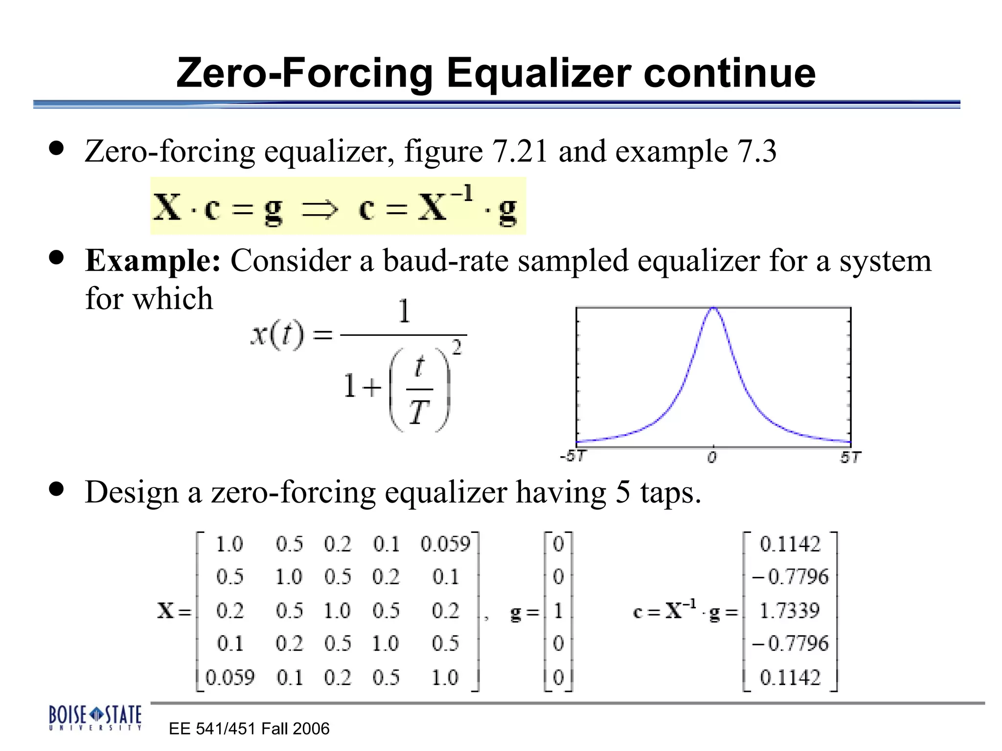
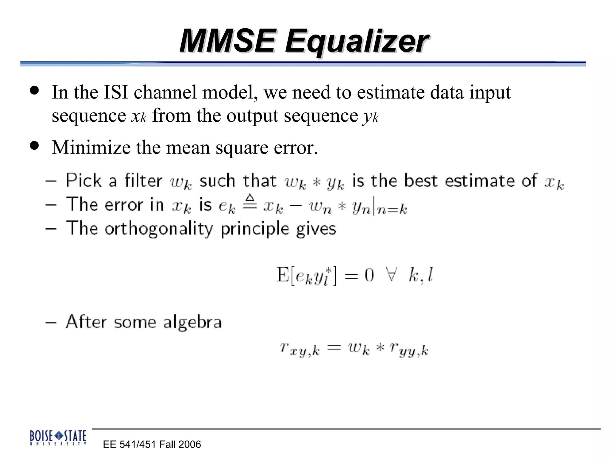
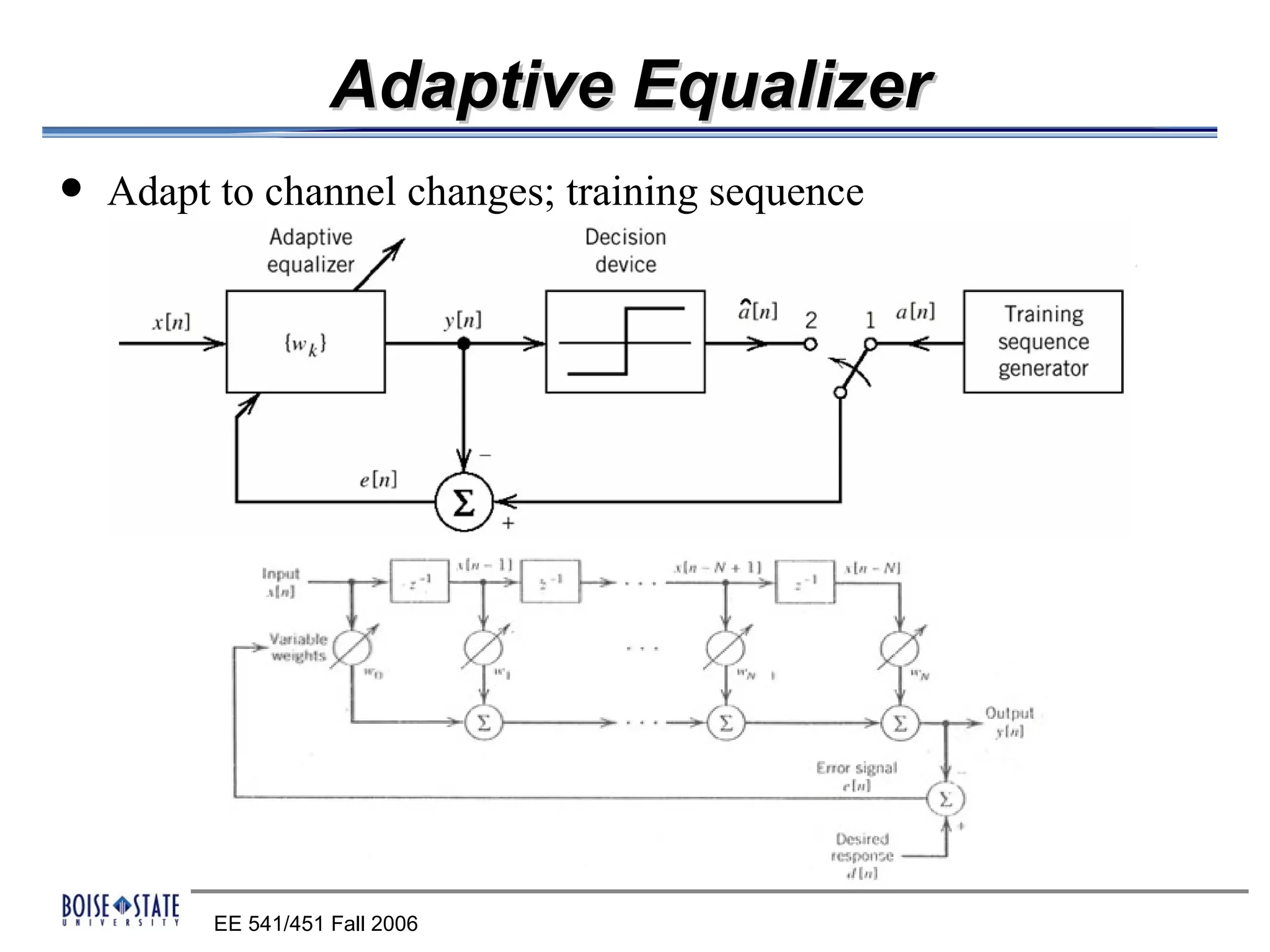
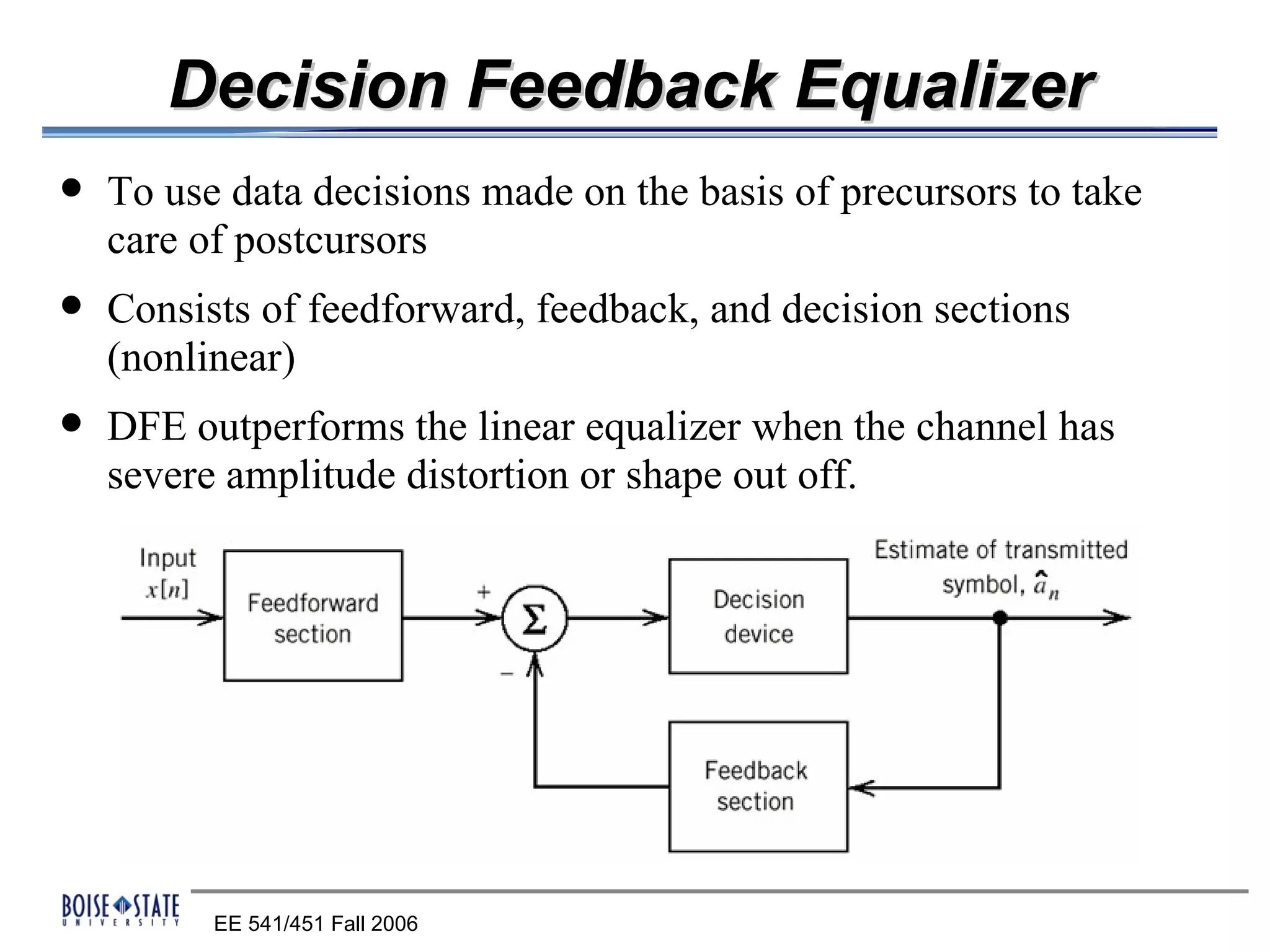
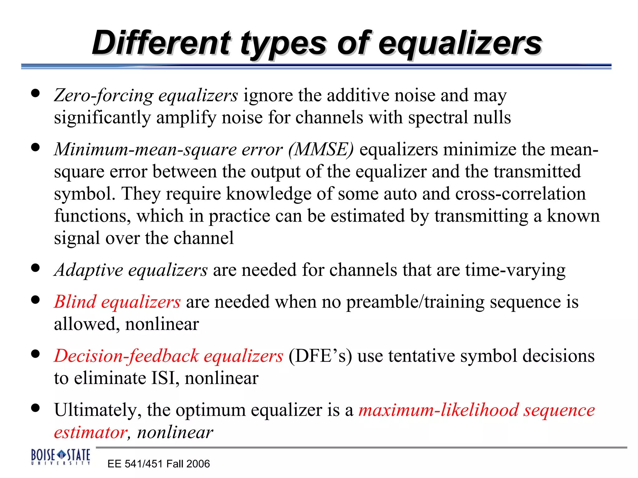
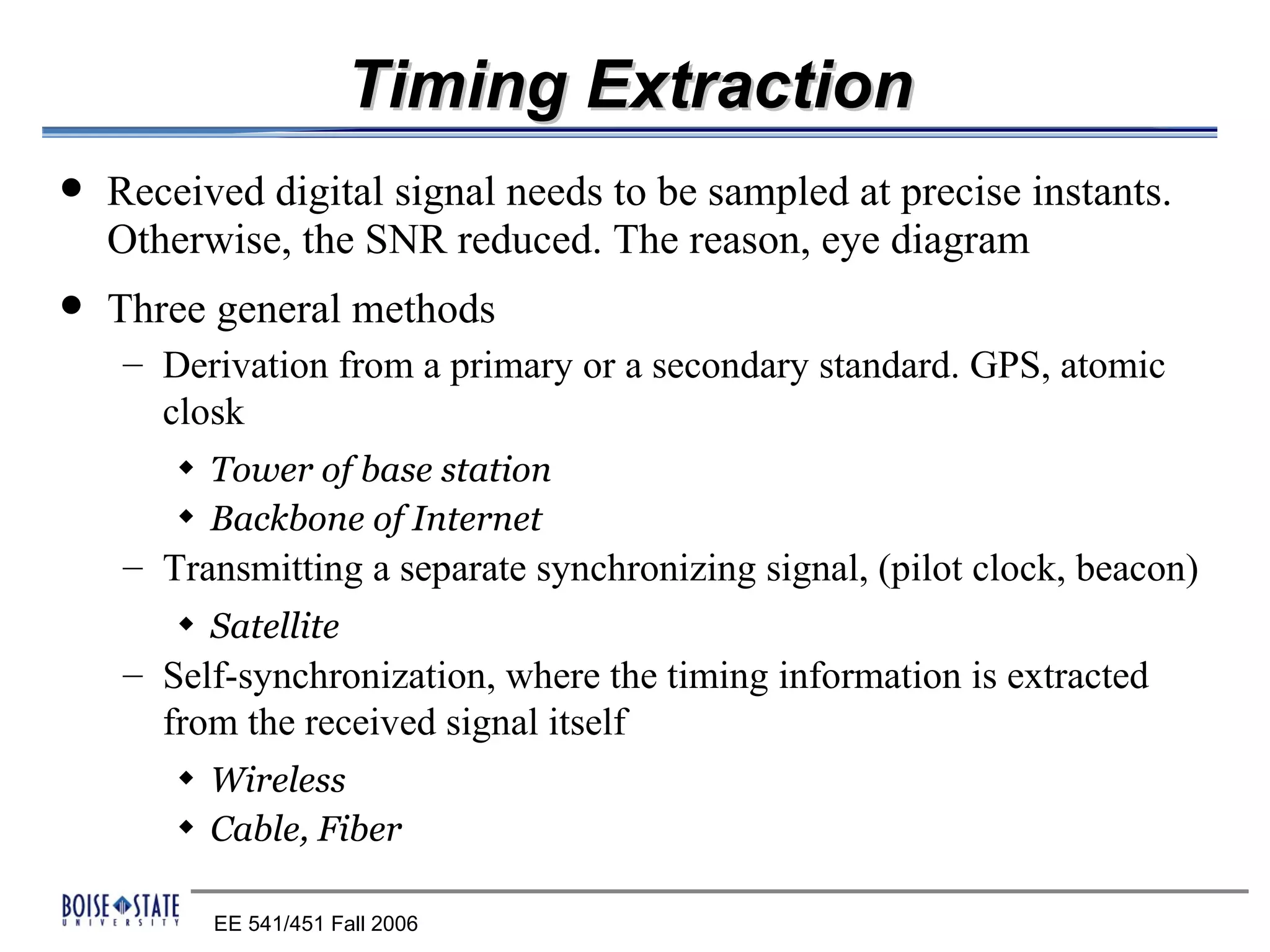
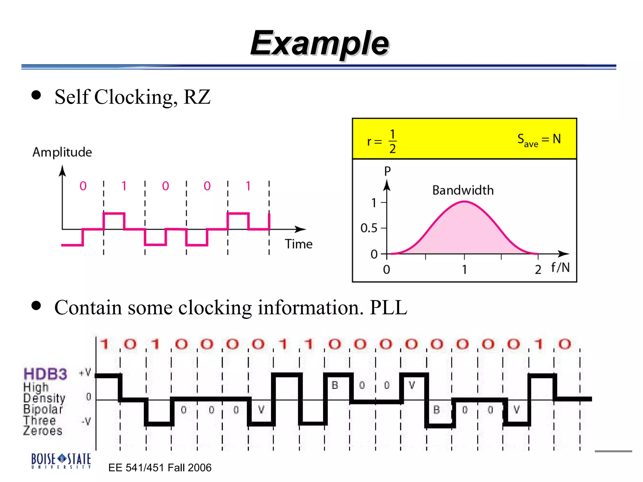
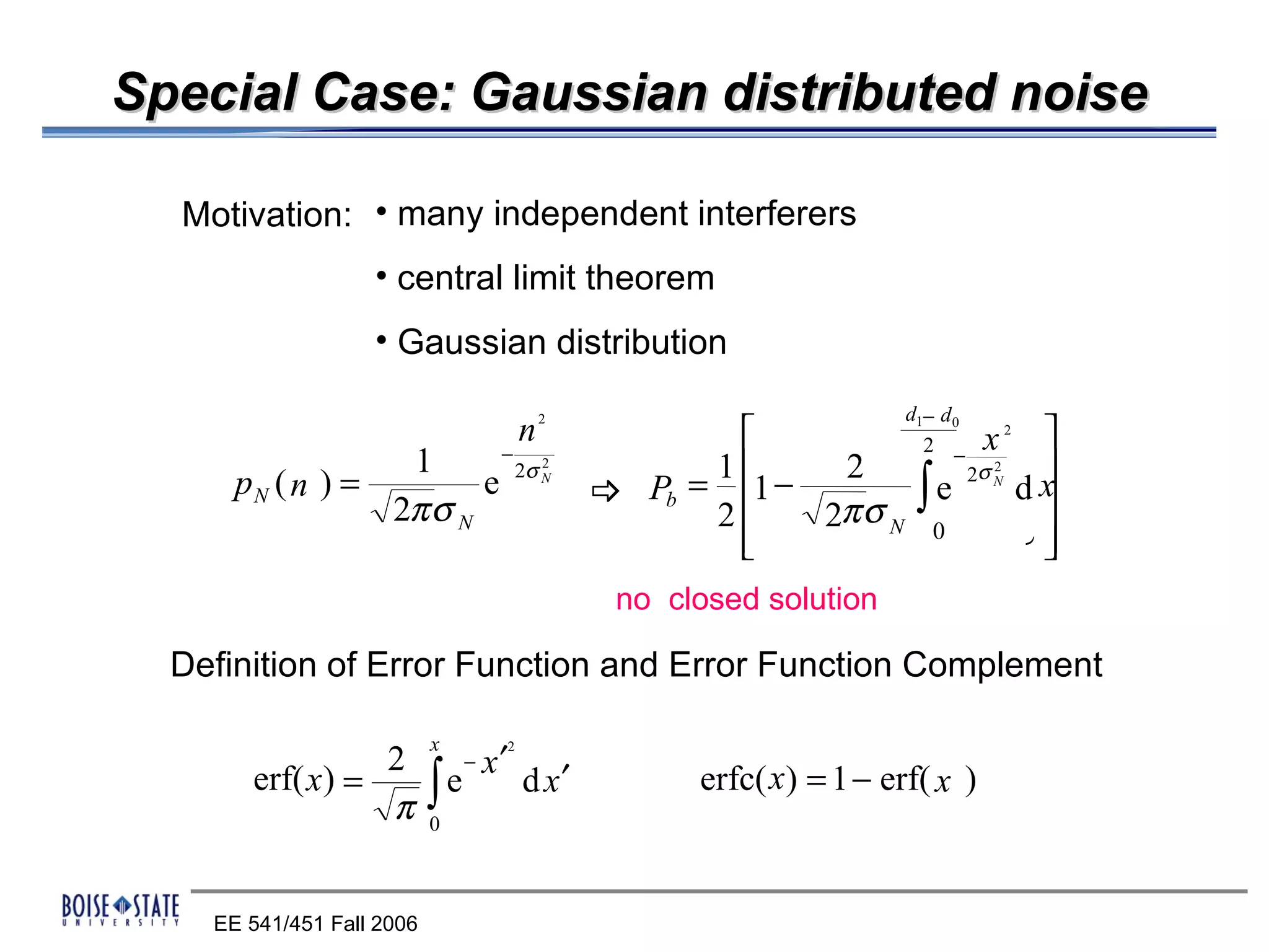
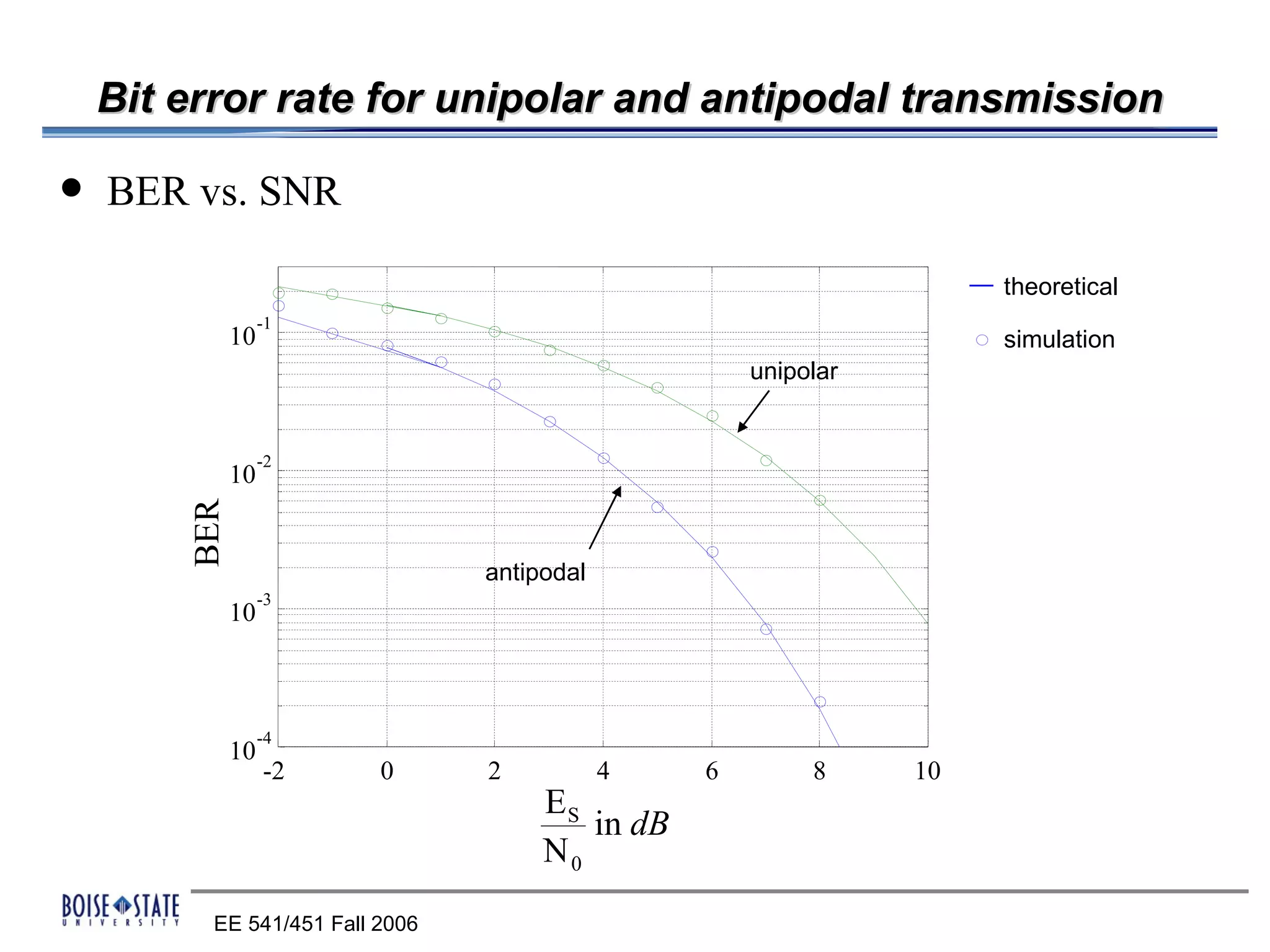
The receiver structure consists of four main components: 1. A matched filter that maximizes the SNR by matching the source impulse and channel. 2. An equalizer that removes intersymbol interference. 3. A timing component that determines the optimal sampling time using an eye diagram. 4. A decision component that determines whether the received bit is a 0 or 1 based on a threshold. The performance of the receiver depends on factors like noise, equalization technique used, and timing accuracy. The bit error rate can be estimated using tools like error functions.

1. Receiver Structure
 Matched filter: match source impulse and maximize SNR
– grx to maximize the SNR at the sampling time/output
 Equalizer: remove ISI
 Timing
– When to sample. Eye diagram
 Decision
– d(i) is 0 or 1 Figure 7.20
Noise na(t)
i ⋅T
d(i) gTx(t) gRx(t) r (iT ) = r0 (iT ) + n(iT )
S
→ max
? N
EE 541/451 Fall 2006

2. Matched Filter
 Input signal s(t)+n(t)
 Maximize the sampled SNR=s(T0)/n(T0) at time T0
EE 541/451 Fall 2006

3. Matched filter example
 Received SNR is maximized at time T0
S
Matched Filter: optimal receive filter for maximized
N
example:
gTx (t ) gTx (−t ) gTx (T0 − t ) = g Rx (t )
T0 t T0 t T0 t
transmit filter receive filter
(matched)
EE 541/451 Fall 2006

4. Equalizer
 When the channel is not ideal, or when signaling is not Nyquist,
There is ISI at the receiver side.
 In time domain, equalizer removes ISR.
 In frequency domain, equalizer flat the overall responses.
 In practice, we equalize the channel response using an equalizer
EE 541/451 Fall 2006

5. Zero-Forcing Equalizer
 The overall response at the detector input must satisfy Nyquist’s
criterion for no ISI:
 The noise variance at the output of the equalizer is:
– If the channel has spectral nulls, there may be significant noise
enhancement.
EE 541/451 Fall 2006

6. Transversal Transversal Zero-Forcing Equalizer
 If Ts<T, we have a fractionally-spaced equalizer
 For no ISI, let:
EE 541/451 Fall 2006

7. Zero-Forcing Equalizer continue
 Zero-forcing equalizer, figure 7.21 and example 7.3
 Example: Consider a baud-rate sampled equalizer for a system
for which
 Design a zero-forcing equalizer having 5 taps.
EE 541/451 Fall 2006

8. MMSE Equalizer
 In the ISI channel model, we need to estimate data input
sequence xk from the output sequence yk
 Minimize the mean square error.
EE 541/451 Fall 2006

9. Adaptive Equalizer
 Adapt to channel changes; training sequence
EE 541/451 Fall 2006

10. Decision Feedback Equalizer
 To use data decisions made on the basis of precursors to take
care of postcursors
 Consists of feedforward, feedback, and decision sections
(nonlinear)
 DFE outperforms the linear equalizer when the channel has
severe amplitude distortion or shape out off.
EE 541/451 Fall 2006

11. Different types of equalizers
 Zero-forcing equalizers ignore the additive noise and may
significantly amplify noise for channels with spectral nulls
 Minimum-mean-square error (MMSE) equalizers minimize the mean-
square error between the output of the equalizer and the transmitted
symbol. They require knowledge of some auto and cross-correlation
functions, which in practice can be estimated by transmitting a known
signal over the channel
 Adaptive equalizers are needed for channels that are time-varying
 Blind equalizers are needed when no preamble/training sequence is
allowed, nonlinear
 Decision-feedback equalizers (DFE’s) use tentative symbol decisions
to eliminate ISI, nonlinear
 Ultimately, the optimum equalizer is a maximum-likelihood sequence
estimator, nonlinear
EE 541/451 Fall 2006

12. Timing Extraction
 Received digital signal needs to be sampled at precise instants.
Otherwise, the SNR reduced. The reason, eye diagram
 Three general methods
– Derivation from a primary or a secondary standard. GPS, atomic
closk
x Tower of base station
x Backbone of Internet
– Transmitting a separate synchronizing signal, (pilot clock, beacon)
x Satellite
– Self-synchronization, where the timing information is extracted
from the received signal itself
x Wireless
x Cable, Fiber
EE 541/451 Fall 2006

13. Example
 Self Clocking, RZ
 Contain some clocking information. PLL
EE 541/451 Fall 2006

14. Timing/Synchronization Block Diagram
 Figure 2.3
 After equalizer, rectifier and clipper
 Timing extractor to get the edge and then amplifier
 Train the phase shifter which is usually PLL
 Limiter gets the square wave of the signal
 Pulse generator gets the impulse responses
EE 541/451 Fall 2006

15. Timing Jitter
 Random forms of jitter: noise, interferences, and mistuning of
the clock circuits.
 Pattern-dependent jitter results from clock mistuning and,
amplitude-to-phase conversion in the clock circuit, and ISI,
which alters the position of the peaks of the input signal
according to the pattern.
 Pattern-dependent jitter propagates
 Jitter reduction
– Anti-jitter circuits
– Jitter buffers
– Dejitterizer
EE 541/451 Fall 2006

16. Bit Error Probability
Noise na(t)
i ⋅T
d(i) gTx(t) gRx(t) r0 (i T ) + n(iT )
We assume: • binary transmission with d (i ) ∈ {d 0 , d1}
• transmission system fulfills 1st Nyquist criterion
• noise n(iT), independent of data source
p N (n )
Probability density function (pdf) of n(iT)
Mean and variance
n
EE 541/451 Fall 2006

17. Conditional pdfs
The transmission system induces two conditional pdfs depending on d (i )
• if d (i ) = d 0 • if d (i ) = d1
p0 ( x ) = p N ( x − d 0 ) p1 ( x) = p N ( x − d1 )
p0 ( x ) p1 ( x)
x
d0 d1 x
EE 541/451 Fall 2006

18. Probability of wrong decisions
Placing a threshold S
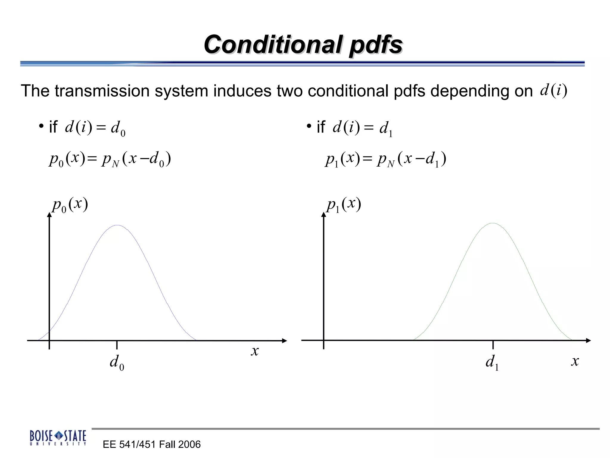
p0 ( x ) p1 ( x)
Probability of
wrong decision
x x
d0 S S d1
∞ S
Q0 = ∫ p0 ( x) dx Q1 =
∫ p ( x)dx
1
S −∞
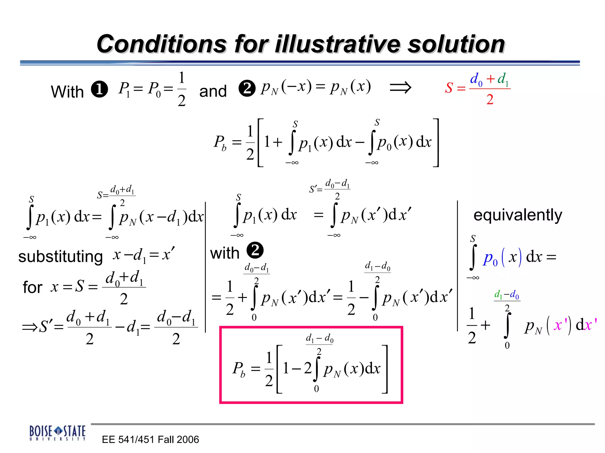
When we define P0 and P1 as equal a-priori probabilities of d 0 and d1
(P0 = P = 1 )
we will get the bit error probability 1 2
∞ S S
Pb = P0Q0 + P Q1 =
1
1
2 ∫s p ( x)dx + ∫ p ( x)dx =
S
0
1
2
−∞
1
1
2 + ∫[
−∞
1
2 p1 ( x) − 1 p0 ( x ) ] dx
2
1 24
4 3
S
1− ∫ p0 ( x ) dx
−∞
EE 541/451 Fall 2006

19. Conditions for illustrative solution
1 d 0 + d1
With  P1 = P0 = and  pN (− x) = pN ( x) ⇒ S=
2
2
S
1 
S
Pb = 1 + ∫ p1 ( x) dx − ∫ p0 ( x ) dx 
2  −∞ −∞ 
d 0 − d1
d +d S ′=
S S= 0 1 S 2
2
∫ p ( x) dx = ∫ p
1 N ( x − d1 )dx ∫ p ( x) dx
1 = ∫p N ( x ′ )d x ′ equivalently
−∞ −∞ −∞ −∞ S
with 
substituting x −d1 = x ′ d −d d −d ∫ p0 ( x ) dx =
d +d
0 1 1 0
2 −∞
for x =S = 0 1 1 2 1
2 = + ∫ p N ( x ′ )d x ′ = − ∫ p N ( x ′ )d x ′ d1 − d 0
d 0 + d1 d 0− d 1 2 0 2 0 1 2
⇒S ′ = − d1= + ∫ p N ( x ' ) dx '
2 2 d −d 1 0 2 0
1 2

Pb = 1 − 2 ∫ p N ( x )dx 
2 0 
EE 541/451 Fall 2006

20. Special Case: Gaussian distributed noise
Motivation: • many independent interferers
• central limit theorem
• Gaussian distribution
d1− d 0
n 2
 x 
2 −
2
−
1 1 2 
e 2σ ∫
2
2σ
pN ( n ) =
2
N
 Pb = 1 − e dx

N
2π σ N 2 2π σ N 0 0

 1 24 
4 3
no closed solution
Definition of Error Function and Error Function Complement
x
2 − x′
2
erf( x) = ∫ e d x′
π 0
erfc( x) = 1 − erf( x )
EE 541/451 Fall 2006

21. Error function and its complement
 function y = Q(x)
y = 0.5*erfc(x/sqrt(2));
2.5
erf(x)
erfc(x)
2
1.5
erf(x), erfc(x)
1
0.5
0
-0.5
-1
-1.5
-3 -2 -1 0 1 2 3
x
EE 541/451 Fall 2006

22. Bit error rate with error function complement
 d1 − d 0
x2 
1 2 1 2 −
 1  d − d0 
∫
2
2σ N
Pb = 1 − e d x  Pb = erfc 1 
2

π 2σ N 0 
2  2 2σ N 
 
Expressions with E S and N 0
antipodal: d1 = + d ; d 0 = − d unipolar d1= + d ; d 0 = 0
1  d −d  1  d  1  d  1  d2 
Pb = erfc  1 0  = erfc   Pb = erfc 
 2 2σ  = erfc 
 2 
2  2 2σ  2  2σ  2  8σ N
2 
 N   N   N   
1  d2  1  SNR  1  d2 / 2  1  SNR 
= erfc   = erfc 
  = erfc   = erfc  
2  2σ N

2  2
  2  2  4σ N  2
2 
 4 
 
d2 ES d2 / 2 ES
SNR = 2 = SNR = 2 =
σN matched N / 2
0 σ N matched N 0 / 2
1  ES  1  ES 
Pb = erfc
 N  Q function Pb = erfc  
2  0  2  2 N0 
 
EE 541/451 Fall 2006

23. Bit error rate for unipolar and antipodal transmission
 BER vs. SNR
theoretical
-1
10 simulation
unipolar
-2
10
BER
antipodal
-3
10
-4
10
-2 0 2 4 6 8 10
ES
in dB
N0
EE 541/451 Fall 2006