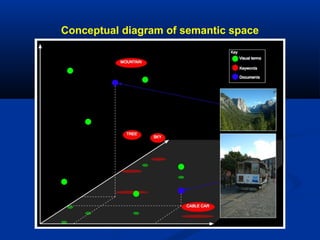
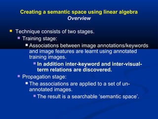
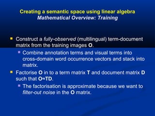
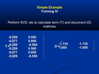
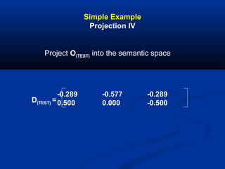
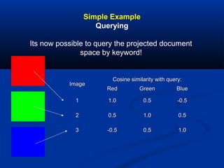
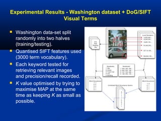
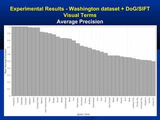
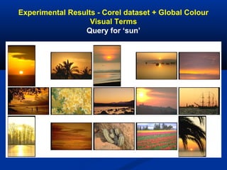
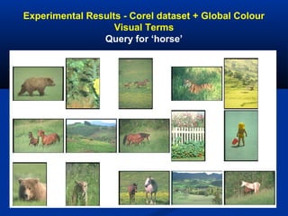
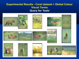
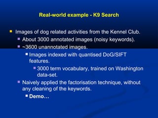
The document discusses multimodal searching and semantic spaces to enhance image retrieval, particularly for unannotated images. It explores computational and mathematical techniques like latent semantic indexing to enable content-based multimedia search without relying on extensive metadata. Experimental results demonstrate the effectiveness of these methods in various datasets, including applications for kennel club imagery.

1. Multimodal Searching and
Semantic Spaces
…or how to find images of Dalmatians
when there is no metadata
Jonathon Hare

2. Contents
 Introduction
 The problem: un-annotated images
 A brief introduction to textual information techniques: Bags-of-
words, the Vector-space model and Latent Semantic Indexing
 The image-to-semantics pipeline
 Modelling image content
 Visual terms and the bag-of-words for image content
 Semantic-Spaces
 Problems associated with auto-annotation w.r.t search
 Underlying theory and justification
 A simple example
 Experimental results
 K9 Search demo
 Wrap-up

3. Introduction
 The previous sessions have described the issues associated with
image retrieval from the practitioner perspective -- a problem that
has become known as the ‘semantic gap’ in image retrieval.
 In the previous session, Criss described a number of techniques for
improving the ability to search image collections using thesauri and
ontological techniques.
 Unfortunately, these techniques require the image collection to
be extensively annotated.
 This final session aims to explore how the use of novel
computational and mathematical techniques can be used to help
improve content-based multimedia search by enabling textual
search of un-annotated imagery.

4. Un-annotated Imagery
 Manually constructing metadata in order to index
images is expensive.
 Estimates of US$50-$100 per image for the
level of detail involved in a typical Getty
archival image (keywords, caption, title,
description, dates, times, events).
 Every day, the number of images is
increasing.
 In many domains, manually indexing
everything is an impossible task!

5. Un-annotated Imagery - Example
 Kennel club image collection.
 relatively small (~60,000 images)
 ~7000 of those digitised.
 ~3000 of those have subject metadata (mostly
keywords), remainder have no information.
 Each year, after the Crufts dog show they
expect to receive an additional 4000-8000
(digital) images with no metadata other than
date/time (and only then if the camera is set-up
correctly)

6. A brief introduction to (textual) information retrieval
techniques
 “Information retrieval (IR) is the art and science of searching for
information in documents, searching for documents themselves,
searching for metadata which describe documents, or searching
within databases, whether relational stand alone databases or
hypertext networked databases such as the Internet or intranets, for
text, sound, images or data.” --wikipedia
Traditionally in IR, documents represented as sets/bags of terms.
 Bag: allows multiple instances of the same term.
 terms normally equate to words in the document.
 Document structure ignored.
 Commonly used terms (stop words) often ignored.

7. Bag of Words Example
The quick brown
fox jumped over
the lazy dog’s
back.
Document 1
Document 2
Now is the time
for all good men
to come to the
aid of their party.
the
quick
brown
fox
over
lazy
dog
back
now
is
time
for
all
good
men
to
come
jump
aid
of
their
party
0
0
1
1
0
1
1
0
1
1
0
0
1
0
1
0
0
1
1
0
0
1
0
0
1
0
0
1
1
0
1
0
1
1
Indexed
Term
Document1
Document2
Stop Word
List
‘s
courtesy of Phillip Resnik

8. Vector-space model
 A collection of n documents with t distinct terms can be represented
by a (sparse) matrix.
 Documents are row vectors of the matrix.
 Elements, w, are a function of the number of times term i occurs
in document j.
 A query can also be represented as a vector like a document.
T1 T2 … Tt
D1 w11 w21 … wt1
D2 w12 w22 … wt2
: : : :
: : : :
Dn w1n w2n … wtn

9. Documents as Vectors
Star
Diet
Doc about astronomy
Doc about movie stars
Doc about mammal behavior

10. Geometric Interpretation
Example:
D1 = 2T1 + 3T2 + 5T3
D2 = 3T1 + 7T2 + T3
Q = 0T1 + 0T2 + 2T3
T3
T1
T2
D1 = 2T1+ 3T2 + 5T3
D2 = 3T1 + 7T2 + T3
Q = 0T1 + 0T2 + 2T3
7
32
5
• Is D1 or D2 more similar to Q?
• How to measure the degree of
similarity? Distance? Angle?
Projection?
Assumption: Documents that are “close together”
in space are similar in meaning.

11. Cosine Similarity
 Most popular measure of similarity between the query and
document vectors is the cosine similarity measure.
 …the cosine of angle between the vectors.
 Value of 1.0 means document and query are identical.
 Distance metric easily obtained by taking cos-1
(similarity).
Q• D
|Q |
1
2
× | D |
1
2

12. Latent Semantic Indexing/Analysis
 A problem with the Vector-space model is that it relies on
lexical matching.
 A search for ‘automobile’ would not find documents about
‘cars’.
 Doesn’t deal with synonymy (multiple terms with the
same meaning), or polysemy (words with multiple
meanings).
 Latent Semantic Indexing is a technique that attempts to take
advantage of implicit higher-order structure in the term-
document matrix in order to circumvent this problem.
 Works by reducing the dimensionality of the vector-space
in order to bring similar terms and documents closer
together.

13. Latent Semantic Indexing: Dimensionality Reduction

14. Latent Semantic Indexing: How does it work?
 Definition: Rank of a matrix is the number of linearly
independent rows or columns of that matrix.
 Some intuition: Given a large enough corpus, many
terms or documents in a given term-document matrix will
be linearly dependent.
 i.e. the “Cat” and “Feline” term columns will be
approximately linearly dependent on each other!
 …So, all we need do is estimate a lower-rank version of
the original term-document matrix.

15. Latent Semantic Indexing: Mathematical details
 LSI uses a matrix decomposition called the Singular Value
Decomposition (SVD).
 SVD decomposes a matrix A into three separate matrices U, ∑,
and V, such that:
 The decomposition has some nice properties, in particular, ∑ is
a diagonal matrix containing the so-called singular values of A in
monotonically decreasing order. The decomposition also
separates the documents and terms into vector separate spaces
(U and V respectively, both to each other by ∑).
 It can be shown that by selecting the K largest singular values
and corresponding left and right vectors it is possible to estimate
the rank K version of A with minimum error (in the least-squares
sense).
A = UΣVT

16. Latent Semantic Indexing: Mathematical Details
Note: In practice it isn’t necessary to reconstruct
Ak. The term vectors in U and document vectors in
V can be used directly.

17. Typical Information Flow from Raw Media to Semantics

18. Modelling visual information
 In order to model the visual content of an image we can
generate and extract descriptors or feature-vectors.
 Feature-vectors can describe many differing aspects of the
image content.
 Low level features:
 Fourier transforms, wavelet decomposition, texture
histograms, colour histograms, shape primitives, filter
primitives, etc.
 Higher-level features:
 Faces, objects, etc.

19. Visual Term Representations
 The text indexing approaches described earlier use a bag-of-terms
approach, whereby the documents are split into a vector counting
the occurrences of the individual components.
 It is possible to represent purely visual information in the same
way, using feature vectors.
 Some feature-vectors which are continuous may need to be
quantised into discrete visual terms.

20. Global Colour Visual Terms
 A common way of indexing the global colours used in an
image is the colour histogram.
 The each bin of the histogram counts the number of
pixels of the colour range represented by that bin.
 The colour histogram can thus be used directly as a
term occurrence vector in which each bin is
represented as a visual term.

21. DoG/SIFT Visual Terms
 Features based on
Lowe’s difference-of-
Gaussian region detector
and SIFT feature vector.
 A vocabulary of exemplar
feature-vectors is learnt
by applying k-means
clustering to a training set
of features.
 Feature-vectors can then
be quantised to discrete
visual terms by finding the
closest exemplar in the
vocabulary.

22. Semantic Spaces
 Idea based on a technique from text retrieval known as
cross-language latent semantic indexing.
 Extension of standard latent semantic indexing into
multiple languages.
 Combines image content indexed as ‘visual’ terms with
textual terms in the same term-occurrence vector.
 Basically, just a big vector-space where the
documents are images (or any kind of media) and
terms from multiple
languages/vocabularies/modalities are used.

23. Conceptual diagram of semantic space

24. Creating a semantic space using linear algebra
Overview
 Technique consists of two stages.
 Training stage:
 Associations between image annotations/keywords
and image features are learnt using annotated
training images.
 In addition inter-keyword and inter-visual-
term relations are discovered.
 Propagation stage:
 The associations are applied to a set of un-
annotated images.
 The result is a searchable ‘semantic space’.

25. Creating a semantic space using linear algebra
Mathematical Overview: Training
 Construct a fully-observed (multilingual) term-document
matrix from the training images O.
 Combine annotation terms and visual terms into
cross-domain word occurrence vectors and stack into
matrix.
 Factorise O in to a term matrix T and document matrix D
such that O≈TD.
 The factorisation is approximate because we want to
filter-out noise in the O matrix.

26. Creating a semantic space using linear algebra
Hang on! What do we mean by noise?
 Consider the following noise-free term document matrix with two
documents and two terms. The first term is the keyword “Red”, and
the second represents a visual term - the RGB triple {255, 0, 0}.
 The matrix has rank 1, indicating that the terms “Red” and “{255, 0,
0}” are equivalent (as are Doc. 1 and Doc. 2).
 Of course, in reality the matrix is not this clean, and so some form of
filtering needs to be performed to match-up the relationships.

27. Creating a semantic space using linear algebra
So how do we filter and perform the factorisation?
 Simple!
 The solution to the filtering and factorisation problem is simple:
Use the Singular Value Decomposition and throw away all but
the K most important singular values.
 Just like in LSI
 also closely related to Tomasi-Kanade factorisation for
structure-from-motion.

28. Creating a semantic space using linear algebra
But hang-on, doesn’t SVD give you 3 matrices?
 SVD gives you three matrices; P=U∑VT
 However, we can take the K-subspace first two and
multiply them together to get the T matrix.
 T = UK∑K
 The K-subspace of the third matrix forms D.
 D = VT
K

29. Creating a semantic space using linear algebra
Mathematical Overview: Training II
 The T matrix tells us how terms are inter-related - each
term forms a point in a vector-space, with the
coordinates given by the relevant row of T.
 The D matrix tells us how documents (images) are inter-
related - each term forms a point in a vector-space, with
the coordinates given by the relevant column of D.
 Together, the T and D matrices capture the relationships
between the terms and documents.
O≈TD

30. Creating a semantic space using linear algebra
Mathematical Overview: Propagation
 In order to propagate the associations learnt in the
training stage to un-annotated images, the T matrix can
be used to project a partially observed term-document
matrix, P, into the space defined by T thus creating a
new document matrix Δ.
 It can be shown that to solve for Δ, it is simply a matter
of pre-multiplying the transpose of T with P.
P=TΔ
Δ=TT
P

31. Creating a semantic space using linear algebra
Mathematical Overview: Searching
 We now have two matrices:
 T which contains the coordinates of each term is a
semantic space,
 and Δ, which contains the coordinates of each un-
annotated image/document in the same semantic
space.
 So, in essence, we have a vector-space of terms and
documents which can be searched using standard
techniques.
 i.e. ranking documents using cosine similarity to a
query term.

32. Simple Example
Training I
Annotated Training Images
Red, Green Green, Blue

33. Simple Example
Training II
Simple feature-vector/visterms representing dominant primary
colours
{255,0,0},{0,255,0} {0,255,0}, {0,0,255}

34. Simple Example
Training III
Construct Term-Document Matrix O(TRAIN):
O(TRAIN) =
1 0
1 1
0 1
1 0
1 1
0 1
Image#1Image#2
Red
Green
Blue
{255,0,0}
{0,255,0}
{0,0,255}

35. Simple Example
Training IV
T =
-0.289 0.500
-0.577 0.000
-0.289 -0.500
-0.289 0.500
-0.577 0.000
-0.289 -0.500
Perform SVD, etc to calculate term (T) and document (D)
matrices
-1.735 -1.735
1.000 -1.000D =

36. Simple Example
Projection I
Un-annotated Testing Images

37. Simple ExampleSimple Example
Projection IIProjection II
Simple feature-vector/visterms representing dominant
primary colours
{255,0,0} {0,255,0} {0,0,255}

38. Simple Example
Projection III
O(TEST) =
0 0 0
0 0 0
0 0 0
1 0 0
0 1 0
0 0 1
Image#1Image#2
Red
Green
Blue
{255,0,0}
{0,255,0}
{0,0,255}
Construct Term-Document Matrix O(TEST):
Image#3

39. Simple Example
Projection IV
Project O(TEST) into the semantic space
-0.289 -0.577 -0.289
0.500 0.000 -0.500D(TEST) =

40. Simple Example
Querying
Its now possible to query the projected document
space by keyword!
ImageImage
Cosine similarity with query:Cosine similarity with query:
RedRed GreenGreen BlueBlue
11 1.01.0 0.50.5 -0.5-0.5
22 0.50.5 1.01.0 0.50.5
33 -0.5-0.5 0.50.5 1.01.0

41. Experimental Results - Washington dataset + DoG/SIFT
Visual Terms
 Washington data-set split
randomly into two halves
(training/testing).
 Quantised SIFT features used
(3000 term vocabulary).
 Each keyword tested for
retrieving relevant images
and precision/recall recorded.
 K value optimised by trying to
maximise MAP at the same
time as keeping K as small as
possible.

42. Experimental Results - Washington dataset + DoG/SIFT
Visual Terms
Average Precision

43. Experimental Results - Corel dataset + Global Colour
Visual Terms
 RGB Histograms used as visual terms (each bin
representing a single term).
 Standard collection: 500 test images, 4500 training
images.
 Results quite impressive >> than Machine Translation
auto-annotation technique (but remember we are using
much simpler image features).
 Works well for query keywords that are easily
associated with a particular set of colours,
 but not so well for the other keywords.

44. Experimental Results - Corel dataset + Global Colour
Visual Terms
Query for ‘sun’

45. Experimental Results - Corel dataset + Global Colour
Visual Terms
Query for ‘horse’

46. Experimental Results - Corel dataset + Global Colour
Visual Terms
Query for ‘foals’

47. Real-world example - K9 Search
 Images of dog related activities from the Kennel Club.
 About 3000 annotated images (noisy keywords).
 ~3600 unannotated images.
 Images indexed with quantised DoG/SIFT
features.
 3000 term vocabulary, trained on Washington
data-set.
 Naively applied the factorisation technique, without
any cleaning of the keywords.
 Demo…