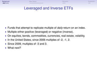
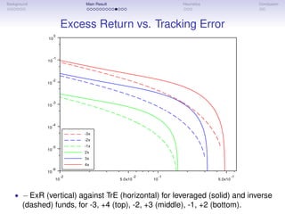
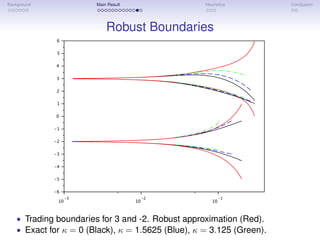
Background Main Result Heuristics Conclusion
Leveraged ETFs:
Robust Replication and Performance Evaluation
Paolo Guasoni1,2
Eberhard Mayerhofer2,3
Boston University1
Dublin City University2
University of Limerick3
Byrne Workshop on Stochastic Analysis in Finance and Insurance
June 6th
, 2016
Background Main Result Heuristics Conclusion
Outline
• Motivation:
Leveraged ETFs: Tracking Error vs. Excess Return.
• Model:
Optimal Tracking with Trading Costs.
Volatility process stationary.
• Results:
Optimal Tracking Policy.
Optimal Tradeoff between Tracking Error and Excess Return.
Background Main Result Heuristics Conclusion
Leveraged and Inverse ETFs
• Funds that attempt to replicate multiple of daily return on an index.
• Multiple either positive (leveraged) or negative (inverse).
• On equities, bonds, commodities, currencies, real estate, volatility.
• In the United States, since 2006 multiples of -2, -1, 2.
• Since 2009, multiples of -3 and 3.
• What next?
Background Main Result Heuristics Conclusion
6, 8, 10, 15 since 2016 in Germany
Background Main Result Heuristics Conclusion
Simple – In principle
• If index follows
dSt
St
− rt dt = µt dt + σt dWt
• Then leveraged or inverse ETF is portfolio with constant proportion Λ
dwt
wt
− rt dt = Λµt dt + Λσt dWt
• Fund price
wt = w0 exp
t
0
rsds + Λ
t
0
µsds −
Λ2
2
t
0
σ2
s ds + Λ
t
0
σsdWs
• Compounding implies Volatility decay: when the multiple Λ is high, the
fund loses value regardless of the index’s return.
• High expected value, but almost surely going to zero.
• Annual or monthly returns are not multiplied.
• From a frictionless viewpoint, risky but simple products.
• But when the multiple is high also rebalancing costs are high...
Background Main Result Heuristics Conclusion
Literature
• Compounding:
Avellaneda and Zhang (2010), Jarrow (2010), Lu, Wang, Zhang (2009)
• Rebalancing and Market Volatility:
Cheng and Madhavan (2009), Charupat and Miu (2011).
• Underexposure:
Tang and Xu (2013): “LETFs show an underexposure to the index that
they seek to track.”
• Underperformance:
Jiang and Yan (2012), Avellaneda and Dobi (2012), Guo and Leung
(2014), Wagalath (2014).
• Many authors attribute deviations to frictions. Model?
Background Main Result Heuristics Conclusion
Dilemma
• With costless rebalancing, keep constant leverage. Perfect tracking:
dDt =
dwt
wt
− Λ
dSt
St
+ (Λ − 1)rt dt = 0
• Excess return DT /T and tracking error D T /T both zero.
• With costly rebalancing, dream is broken.
• Rebalancing reduces tracking error but makes deviation more negative.
• Questions:
• What are the optimal rebalancing policies?
• How to compare funds differing in excess return and tracking error?
• Implications:
• Underexposure consistent with optimality?
• Underperformance significant?
Background Main Result Heuristics Conclusion
This Paper
• Model of Optimal Tracking with Trading Costs.
• Excess Return vs. Tracking Error.
• Underlying index follows Îto process. Zero drift in basic model.
• Robust tracking policy: independent of volatility process at first order.
• Excess return and tracking error depend only on average volatility.
• Explains underexposure puzzle.
Background Main Result Heuristics Conclusion
Basic Model
• Filtered probability space (Ω, (Ft )t≥0, F, P) with Brownian motion W and
its augmented natural filtration.
• Safe asset with adapted, integrable rate rt .
• Index with ask (buying) price St :
dSt
St
= rt dt + σt dWt ,
where σ2
t is adapted and integrable, i.e. St is well defined.
• Proportional costs: bid price equals (1 − ε)St .
• Zero excess return assumption:
no incentive to outperform index through extra exposure.
• Main results robust to typical risk premia.
• Stationary volatility: for some ¯σ > 0,
lim
T→∞
1
T
T
0
σ2
t dt = ¯σ2
Background Main Result Heuristics Conclusion
Objective
• Trading strategy:
Number of shares ϕt = ϕ↑
t − ϕ↓
t as purchases minus sales. Fund value:
dXt =rt Xt dt − St dϕ↑
t + (1 − ε)St dϕ↓
t (cash)
dYt =St dϕ↑
t − St dϕ↓
t + ϕt dSt (index)
wt = Xt + Yt . Admissibility: wt ≥ 0 a.s. for all t.
• (Annual) Excess Return:
ExR =
1
T
T
0
dwt
wt
− Λ
dSt
St
+ (Λ − 1)rt dt =
DT
T
• (Annual) Tracking Error:
TrE =
D T
T
• Maximize long term excess return given tracking error:
max
ϕ
lim sup
T→∞
1
T
DT −
γ
2
D T
• Similar to mean-variance tradeoff in portfolio choice.
Background Main Result Heuristics Conclusion
Main Result
Theorem (Exact)
Assume Λ = 0, 1.
i) For any γ > 0 there exists ε0 > 0 such that for all ε < ε0, the system
1
2 ζ2
W (ζ) + ζW (ζ) − γ
(1+ζ)2 Λ − ζ
1+ζ = 0,
W(ζ−) = 0, W (ζ−) = 0,
W(ζ+) = ε
(1+ζ+)(1+(1−ε)ζ+) , W (ζ+) = ε(ε−2(1−ε)ζ+−2)
(1+ζ+)2(1+(1−ε)ζ+)2
has a unique solution (W, ζ−, ζ+) for which ζ− < ζ+.
ii) The optimal policy is to buy at π− := ζ−/(1 + ζ−) and sell at
π+ := ζ+/(1 + ζ+) to keep πt = ζt /(1 + ζt ) within the interval [π−, π+].
iii) The maximum performance is
lim sup
T→∞
DT −
γ
2
D T = −
γσ2
2
(π− − Λ)2
,
Background Main Result Heuristics Conclusion
Main Result (continued)
Theorem (Exact)
iv) Excess return and tracking error:
ExR =
σ2
2
π−π+(π+ − 1)2
(π+ − π−)(1/ε − π+)
TrE = σ π−π+ + Λ(Λ − 2¯β)
where ¯β is the average exposure
¯β := lim
T→∞
· dw
w ,
· dS
S T
· dS
S T
= lim
T→∞
T
0
σ2
t πt dt
T
0
σ2
t dt
= log(π+/π−)
π+π−
π+ − π−
• ODE depends only on multiple Λ and trading cost ε. So do π−, π+.
• ExR and TrE depend also on ¯σ.
Background Main Result Heuristics Conclusion
Main Result
Theorem (Robust Approximation)
• Trading boundaries:
π± = Λ ±
3
4γ
Λ2
(Λ − 1)2
1/3
ε1/3
+ O(ε2/3
)
• Excess return:
ExR = −
3σ2
γ
γΛ(Λ − 1)
6
4/3
ε2/3
+ O(ε)
• Tracking error:
TrE = σ
√
3
Λ(Λ − 1)
6
√
γ
2/3
ε1/3
+ O(ε)
Background Main Result Heuristics Conclusion
The Tradeoff
• Previous formulas imply that
ExR = −
31/3
12
σ3
Λ2
(Λ − 1)2 ε
TrE
+ O(ε4/3
)
• Maximum excess return for given tracking error.
• Equality for optimal policy, otherwise lower excess return. In general:
ExR · TrE ≤ −
31/3
12
σ3
Λ2
(Λ − 1)2
ε + O(ε4/3
)
• Robust formula. Depends on model only through average volatility.
Dynamic irrelevant.
• To evaluate tracking performance of funds on same index, compare
ExR · TrE
σ3
Λ2(Λ − 1)2
• Higher (less negative) is better.
• Comparisons across multiples and over time.
Background Main Result Heuristics Conclusion
Trading Boundaries
• Trading boundaries (vertical) vs.tracking error (horizontal) for leveraged
(solid) and inverse (dashed) funds, for 4 (top), 3, 2, −1, −2, −3 (bottom).
Background Main Result Heuristics Conclusion
Underexposure Explained
• Average exposure:
¯β = Λ −
2Λ − 1
γ
γΛ(Λ − 1)
6
1/3
ε2/3
+ O(ε),
• 0 < ¯β < Λ for leveraged funds.
• Λ < ¯β < 0 for inverse funds.
• Underexposure results from optimal rebalancing.
• Effect increases with multiple and illiquidity.
• Decreases with tracking error.
Background Main Result Heuristics Conclusion
Excess Return vs. Tracking Error
• − ExR (vertical) against TrE (horizontal) for leveraged (solid) and inverse
(dashed) funds, for -3, +4 (top), -2, +3 (middle), -1, +2 (bottom).
Background Main Result Heuristics Conclusion
Robustness to Risk Premium
• Basic model assumes asset with zero risk premium. Does it matter?
• Not at the first order. Not for typical risk premia.
• Extended model. Index price
dSt
St
= (rt + κσ2
t )dt + σt dWt ,
• Manager can generate positive excess return through overexposure.
• But investor observes and controls for overexposure. Objective
lim sup
T→∞
1
T
DT − κ¯β
·
0
dS
S T
−
γ
2
D T
• Effect of κ remains only in state dynamics, not in objective.
• Trading boundaries:
π± = Λ±
3
4γ
Λ2
(Λ − 1)2
1/3
ε1/3
−
(Λ − κ/2)
γ
γΛ(Λ − 1)
6
1/3
ε2/3
+O(ε).
Background Main Result Heuristics Conclusion
Robust Boundaries
• Trading boundaries for 3 and -2. Robust approximation (Red).
• Exact for κ = 0 (Black), κ = 1.5625 (Blue), κ = 3.125 (Green).
Background Main Result Heuristics Conclusion
Robustness to Finite Horizon
• Basic model assumes long horizon. Does it matter?
• Compare by simulation excess returns and tracking errors to
Black-Scholes and Heston models. (µ = 0 (top), 4%, 8% bottom.)
Background Main Result Heuristics Conclusion
Value Function
•
max
ϕ∈Φ
E
T
0
γσ2
t Λπt −
γσ2
t
2
π2
t dt − ε
T
0
πt
dϕ↓
t
ϕt
•
Fϕ
(t) =
t
0
γσ2
s Λ ζs
1+ζs
−
γσ2
s
2
ζ2
s
(1+ζs)2 ds − ε
t
0
ζs
1+ζs
dϕ↓
s
ϕs
+ V(t, ζt )
• Dynamics of Fϕ
by Itô’s formula
dFϕ
(t) = γΛσ2
t
ζt
1 + ζt
−
γσ2
t
2
ζ2
t
(1 + ζt )2
dt − ε
ζt
1 + ζt
dϕ↓
t
ϕt
+ Vt (t, ζt )dt + Vζ(t, ζt )dζt +
1
2
Vζζ(t, ζt )d ζ t ,
• Self-financing condition yields
dζt
ζt
= σt dWt + (1 + ζt )
dϕt
ϕt
+ εζt
dϕ↓
t
ϕt
,
• Whence
dFϕ
(t) = γΛσ2
t
ζt
1 + ζt
−
γσ2
t
2
ζ2
t
(1 + ζt )2
+ Vt +
σ2
t
2
ζ2
t Vζζ dt
Background Main Result Heuristics Conclusion
Control Argument
• Fϕ
(t) supermartingale for any policy ϕ, martingale for optimal policy.
• ϕ↑
and ϕ↓
increasing processes. Supermartingale condition implies
−
ε
(1 + ζ)(1 + (1 − ε)ζ)
≤ Vζ ≤ 0,
• Likewise,
γσ2
t Λ
ζ
1 + ζ
−
γσ2
t
2
ζ2
(1 + ζ)2
+ Vt +
σ2
t
2
ζ2
Vζζ ≤ 0
• For stationary solution, suppose residual value function
V(t, ζ) = λ
T
t
σ2
s ds −
ζ
W(z)dz
• λ to be determined, represents optimal performance over a long horizon
λ
T
T
0
σ2
t dt ≈ λ × σ2
Background Main Result Heuristics Conclusion
Identifying System
• Above inequalities become
0 ≤ W(ζ) ≤
ε
(1 + ζ)(1 + (1 − ε)ζ)
,
γΛ
ζ
1 + ζ
−
γ
2
ζ2
(1 + ζ)2
− λ −
1
2
ζ2
W (ζ) ≤ 0,
• Optimality conditions
1
2
ζ2
W (ζ) − γΛ
ζ
1 + ζ
+
γ
2
ζ2
(1 + ζ)2
+ λ =0 for ζ ∈ [ζ−, ζ+],
W(ζ−) =0,
W(ζ+) =
ε
(ζ+ + 1)(1 + (1 − ε)ζ+)
,
• Boundaries identified by the smooth-pasting conditions
W (ζ−) =0,
W (ζ+) =
ε(ε − 2(1 − ε)ζ+ − 2)
(1 + ζ+)2(1 + (1 − ε)ζ+)2
.
• Four unknowns and four equations.
Background Main Result Heuristics Conclusion
Conclusion
• Optimal tracking of leveraged and inverse funds.
• Excess Return vs. Tracking Error with Frictions.
• Optimal tracking policy independent of volatility dynamics.
• Robust to risk premia and finite horizons.
• Performance depends on volatility only through its average value.
• Sufficient performance statistic: excess return times tracking error.
Background Main Result Heuristics Conclusion
Thank You!
Questions?

Leveraged ETFs Performance Evaluation

  • 1.
    Background Main ResultHeuristics Conclusion Leveraged ETFs: Robust Replication and Performance Evaluation Paolo Guasoni1,2 Eberhard Mayerhofer2,3 Boston University1 Dublin City University2 University of Limerick3 Byrne Workshop on Stochastic Analysis in Finance and Insurance June 6th , 2016
  • 2.
    Background Main ResultHeuristics Conclusion Outline • Motivation: Leveraged ETFs: Tracking Error vs. Excess Return. • Model: Optimal Tracking with Trading Costs. Volatility process stationary. • Results: Optimal Tracking Policy. Optimal Tradeoff between Tracking Error and Excess Return.
  • 3.
    Background Main ResultHeuristics Conclusion Leveraged and Inverse ETFs • Funds that attempt to replicate multiple of daily return on an index. • Multiple either positive (leveraged) or negative (inverse). • On equities, bonds, commodities, currencies, real estate, volatility. • In the United States, since 2006 multiples of -2, -1, 2. • Since 2009, multiples of -3 and 3. • What next?
  • 4.
    Background Main ResultHeuristics Conclusion 6, 8, 10, 15 since 2016 in Germany
  • 5.
    Background Main ResultHeuristics Conclusion Simple – In principle • If index follows dSt St − rt dt = µt dt + σt dWt • Then leveraged or inverse ETF is portfolio with constant proportion Λ dwt wt − rt dt = Λµt dt + Λσt dWt • Fund price wt = w0 exp t 0 rsds + Λ t 0 µsds − Λ2 2 t 0 σ2 s ds + Λ t 0 σsdWs • Compounding implies Volatility decay: when the multiple Λ is high, the fund loses value regardless of the index’s return. • High expected value, but almost surely going to zero. • Annual or monthly returns are not multiplied. • From a frictionless viewpoint, risky but simple products. • But when the multiple is high also rebalancing costs are high...
  • 6.
    Background Main ResultHeuristics Conclusion Literature • Compounding: Avellaneda and Zhang (2010), Jarrow (2010), Lu, Wang, Zhang (2009) • Rebalancing and Market Volatility: Cheng and Madhavan (2009), Charupat and Miu (2011). • Underexposure: Tang and Xu (2013): “LETFs show an underexposure to the index that they seek to track.” • Underperformance: Jiang and Yan (2012), Avellaneda and Dobi (2012), Guo and Leung (2014), Wagalath (2014). • Many authors attribute deviations to frictions. Model?
  • 7.
    Background Main ResultHeuristics Conclusion Dilemma • With costless rebalancing, keep constant leverage. Perfect tracking: dDt = dwt wt − Λ dSt St + (Λ − 1)rt dt = 0 • Excess return DT /T and tracking error D T /T both zero. • With costly rebalancing, dream is broken. • Rebalancing reduces tracking error but makes deviation more negative. • Questions: • What are the optimal rebalancing policies? • How to compare funds differing in excess return and tracking error? • Implications: • Underexposure consistent with optimality? • Underperformance significant?
  • 8.
    Background Main ResultHeuristics Conclusion This Paper • Model of Optimal Tracking with Trading Costs. • Excess Return vs. Tracking Error. • Underlying index follows Îto process. Zero drift in basic model. • Robust tracking policy: independent of volatility process at first order. • Excess return and tracking error depend only on average volatility. • Explains underexposure puzzle.
  • 9.
    Background Main ResultHeuristics Conclusion Basic Model • Filtered probability space (Ω, (Ft )t≥0, F, P) with Brownian motion W and its augmented natural filtration. • Safe asset with adapted, integrable rate rt . • Index with ask (buying) price St : dSt St = rt dt + σt dWt , where σ2 t is adapted and integrable, i.e. St is well defined. • Proportional costs: bid price equals (1 − ε)St . • Zero excess return assumption: no incentive to outperform index through extra exposure. • Main results robust to typical risk premia. • Stationary volatility: for some ¯σ > 0, lim T→∞ 1 T T 0 σ2 t dt = ¯σ2
  • 10.
    Background Main ResultHeuristics Conclusion Objective • Trading strategy: Number of shares ϕt = ϕ↑ t − ϕ↓ t as purchases minus sales. Fund value: dXt =rt Xt dt − St dϕ↑ t + (1 − ε)St dϕ↓ t (cash) dYt =St dϕ↑ t − St dϕ↓ t + ϕt dSt (index) wt = Xt + Yt . Admissibility: wt ≥ 0 a.s. for all t. • (Annual) Excess Return: ExR = 1 T T 0 dwt wt − Λ dSt St + (Λ − 1)rt dt = DT T • (Annual) Tracking Error: TrE = D T T • Maximize long term excess return given tracking error: max ϕ lim sup T→∞ 1 T DT − γ 2 D T • Similar to mean-variance tradeoff in portfolio choice.
  • 11.
    Background Main ResultHeuristics Conclusion Main Result Theorem (Exact) Assume Λ = 0, 1. i) For any γ > 0 there exists ε0 > 0 such that for all ε < ε0, the system 1 2 ζ2 W (ζ) + ζW (ζ) − γ (1+ζ)2 Λ − ζ 1+ζ = 0, W(ζ−) = 0, W (ζ−) = 0, W(ζ+) = ε (1+ζ+)(1+(1−ε)ζ+) , W (ζ+) = ε(ε−2(1−ε)ζ+−2) (1+ζ+)2(1+(1−ε)ζ+)2 has a unique solution (W, ζ−, ζ+) for which ζ− < ζ+. ii) The optimal policy is to buy at π− := ζ−/(1 + ζ−) and sell at π+ := ζ+/(1 + ζ+) to keep πt = ζt /(1 + ζt ) within the interval [π−, π+]. iii) The maximum performance is lim sup T→∞ DT − γ 2 D T = − γσ2 2 (π− − Λ)2 ,
  • 12.
    Background Main ResultHeuristics Conclusion Main Result (continued) Theorem (Exact) iv) Excess return and tracking error: ExR = σ2 2 π−π+(π+ − 1)2 (π+ − π−)(1/ε − π+) TrE = σ π−π+ + Λ(Λ − 2¯β) where ¯β is the average exposure ¯β := lim T→∞ · dw w , · dS S T · dS S T = lim T→∞ T 0 σ2 t πt dt T 0 σ2 t dt = log(π+/π−) π+π− π+ − π− • ODE depends only on multiple Λ and trading cost ε. So do π−, π+. • ExR and TrE depend also on ¯σ.
  • 13.
    Background Main ResultHeuristics Conclusion Main Result Theorem (Robust Approximation) • Trading boundaries: π± = Λ ± 3 4γ Λ2 (Λ − 1)2 1/3 ε1/3 + O(ε2/3 ) • Excess return: ExR = − 3σ2 γ γΛ(Λ − 1) 6 4/3 ε2/3 + O(ε) • Tracking error: TrE = σ √ 3 Λ(Λ − 1) 6 √ γ 2/3 ε1/3 + O(ε)
  • 14.
    Background Main ResultHeuristics Conclusion The Tradeoff • Previous formulas imply that ExR = − 31/3 12 σ3 Λ2 (Λ − 1)2 ε TrE + O(ε4/3 ) • Maximum excess return for given tracking error. • Equality for optimal policy, otherwise lower excess return. In general: ExR · TrE ≤ − 31/3 12 σ3 Λ2 (Λ − 1)2 ε + O(ε4/3 ) • Robust formula. Depends on model only through average volatility. Dynamic irrelevant. • To evaluate tracking performance of funds on same index, compare ExR · TrE σ3 Λ2(Λ − 1)2 • Higher (less negative) is better. • Comparisons across multiples and over time.
  • 15.
    Background Main ResultHeuristics Conclusion Trading Boundaries • Trading boundaries (vertical) vs.tracking error (horizontal) for leveraged (solid) and inverse (dashed) funds, for 4 (top), 3, 2, −1, −2, −3 (bottom).
  • 16.
    Background Main ResultHeuristics Conclusion Underexposure Explained • Average exposure: ¯β = Λ − 2Λ − 1 γ γΛ(Λ − 1) 6 1/3 ε2/3 + O(ε), • 0 < ¯β < Λ for leveraged funds. • Λ < ¯β < 0 for inverse funds. • Underexposure results from optimal rebalancing. • Effect increases with multiple and illiquidity. • Decreases with tracking error.
  • 17.
    Background Main ResultHeuristics Conclusion Excess Return vs. Tracking Error • − ExR (vertical) against TrE (horizontal) for leveraged (solid) and inverse (dashed) funds, for -3, +4 (top), -2, +3 (middle), -1, +2 (bottom).
  • 18.
    Background Main ResultHeuristics Conclusion Robustness to Risk Premium • Basic model assumes asset with zero risk premium. Does it matter? • Not at the first order. Not for typical risk premia. • Extended model. Index price dSt St = (rt + κσ2 t )dt + σt dWt , • Manager can generate positive excess return through overexposure. • But investor observes and controls for overexposure. Objective lim sup T→∞ 1 T DT − κ¯β · 0 dS S T − γ 2 D T • Effect of κ remains only in state dynamics, not in objective. • Trading boundaries: π± = Λ± 3 4γ Λ2 (Λ − 1)2 1/3 ε1/3 − (Λ − κ/2) γ γΛ(Λ − 1) 6 1/3 ε2/3 +O(ε).
  • 19.
    Background Main ResultHeuristics Conclusion Robust Boundaries • Trading boundaries for 3 and -2. Robust approximation (Red). • Exact for κ = 0 (Black), κ = 1.5625 (Blue), κ = 3.125 (Green).
  • 20.
    Background Main ResultHeuristics Conclusion Robustness to Finite Horizon • Basic model assumes long horizon. Does it matter? • Compare by simulation excess returns and tracking errors to Black-Scholes and Heston models. (µ = 0 (top), 4%, 8% bottom.)
  • 21.
    Background Main ResultHeuristics Conclusion Value Function • max ϕ∈Φ E T 0 γσ2 t Λπt − γσ2 t 2 π2 t dt − ε T 0 πt dϕ↓ t ϕt • Fϕ (t) = t 0 γσ2 s Λ ζs 1+ζs − γσ2 s 2 ζ2 s (1+ζs)2 ds − ε t 0 ζs 1+ζs dϕ↓ s ϕs + V(t, ζt ) • Dynamics of Fϕ by Itô’s formula dFϕ (t) = γΛσ2 t ζt 1 + ζt − γσ2 t 2 ζ2 t (1 + ζt )2 dt − ε ζt 1 + ζt dϕ↓ t ϕt + Vt (t, ζt )dt + Vζ(t, ζt )dζt + 1 2 Vζζ(t, ζt )d ζ t , • Self-financing condition yields dζt ζt = σt dWt + (1 + ζt ) dϕt ϕt + εζt dϕ↓ t ϕt , • Whence dFϕ (t) = γΛσ2 t ζt 1 + ζt − γσ2 t 2 ζ2 t (1 + ζt )2 + Vt + σ2 t 2 ζ2 t Vζζ dt
  • 22.
    Background Main ResultHeuristics Conclusion Control Argument • Fϕ (t) supermartingale for any policy ϕ, martingale for optimal policy. • ϕ↑ and ϕ↓ increasing processes. Supermartingale condition implies − ε (1 + ζ)(1 + (1 − ε)ζ) ≤ Vζ ≤ 0, • Likewise, γσ2 t Λ ζ 1 + ζ − γσ2 t 2 ζ2 (1 + ζ)2 + Vt + σ2 t 2 ζ2 Vζζ ≤ 0 • For stationary solution, suppose residual value function V(t, ζ) = λ T t σ2 s ds − ζ W(z)dz • λ to be determined, represents optimal performance over a long horizon λ T T 0 σ2 t dt ≈ λ × σ2
  • 23.
    Background Main ResultHeuristics Conclusion Identifying System • Above inequalities become 0 ≤ W(ζ) ≤ ε (1 + ζ)(1 + (1 − ε)ζ) , γΛ ζ 1 + ζ − γ 2 ζ2 (1 + ζ)2 − λ − 1 2 ζ2 W (ζ) ≤ 0, • Optimality conditions 1 2 ζ2 W (ζ) − γΛ ζ 1 + ζ + γ 2 ζ2 (1 + ζ)2 + λ =0 for ζ ∈ [ζ−, ζ+], W(ζ−) =0, W(ζ+) = ε (ζ+ + 1)(1 + (1 − ε)ζ+) , • Boundaries identified by the smooth-pasting conditions W (ζ−) =0, W (ζ+) = ε(ε − 2(1 − ε)ζ+ − 2) (1 + ζ+)2(1 + (1 − ε)ζ+)2 . • Four unknowns and four equations.
  • 24.
    Background Main ResultHeuristics Conclusion Conclusion • Optimal tracking of leveraged and inverse funds. • Excess Return vs. Tracking Error with Frictions. • Optimal tracking policy independent of volatility dynamics. • Robust to risk premia and finite horizons. • Performance depends on volatility only through its average value. • Sufficient performance statistic: excess return times tracking error.
  • 25.
    Background Main ResultHeuristics Conclusion Thank You! Questions?