The document discusses an optimal investment strategy for stocks, arguing against the commonly advised 'buy and hold' approach in favor of a 'never sell' strategy under certain conditions. It presents a mathematical model that considers transaction costs and dividends, concluding that defining an optimal trading boundary is crucial and that waiting is preferable to selling. The document emphasizes the significance of parameters like risk aversion and investment returns in determining stock trading behavior.

![Outline Model Main Result Implications Heuristics
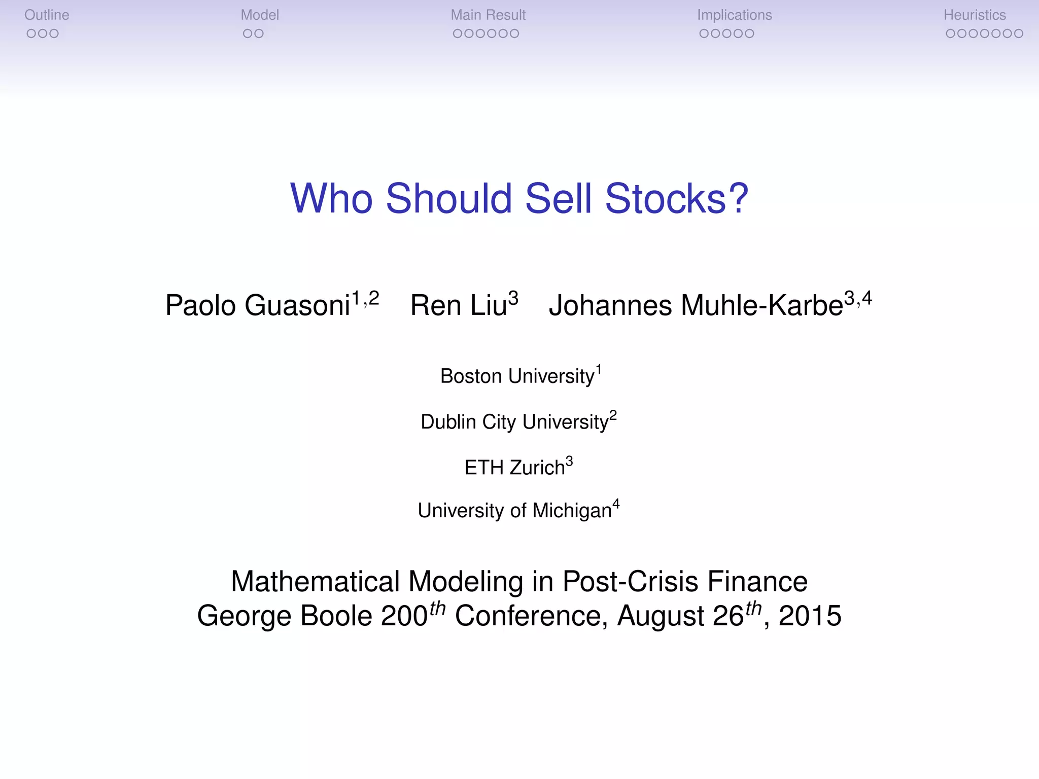
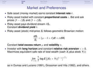
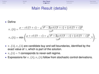
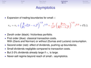
Main Result (Statement)
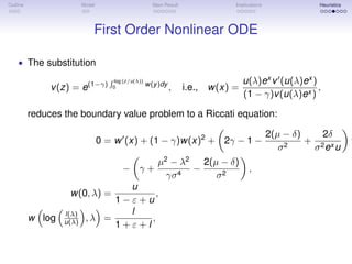
Theorem
Under either condition (CL) or (NS),
• Optimal Strategy:
Hold within (π−, π+). At boundaries, trade to keep the risky weight inside
[π−, π+]. (π− evaluated at ask price (1 + ε)St , π+ at bid (1 − ε)St .)
• Equivalent Safe Rate:
Trading the dividend-paying risky asset with transaction costs equivalent
to leaving all wealth in a hypothetical safe asset that pays the rate
EsR = r +
µ2
− λ2
2γσ2
.
• Reduced value function w(x, λ) has solution in terms of special functions.
• λ does not have closed-form expression. Asymptotics.](https://image.slidesharecdn.com/dividendcork-150826194615-lva1-app6891/85/Who-Should-Sell-Stocks-12-320.jpg)
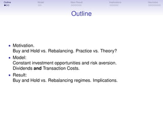
![Outline Model Main Result Implications Heuristics
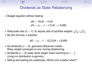
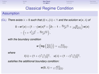
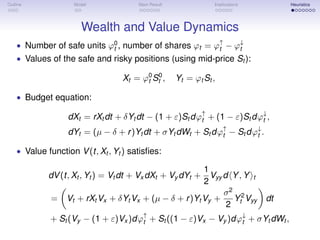
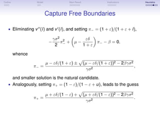
Never Sell. No Regrets.
π∗ optimal never sell buy & hold
[π−, π+] [π−, 1] [0, 1]
50% 1.67% 2.00% 4.67%
60% 1.76% 1.76% 4.41%
70% 1.58% 1.58% 4.21%
80% 1.43% 1.43% 3.81%
90% 1.52% 1.52% 3.70%
• Even when it is not optimal, the never-sell strategy is closer to optimal
than the static buy-and-hold.
• Relative equivalent safe rate loss (EsR0 − EsR)/ EsR0 of optimal
([π−, π+]), never sell ([π−, 1]) and buy-and-hold ([0, 1]) strategies.
• Simulation with T = 20, time step dt = 1/250, and sample N = 2 × 10⁷
.
• µ = 8%, σ = 16%, r = 1%, δ = 2%, and ε = 1%.](https://image.slidesharecdn.com/dividendcork-150826194615-lva1-app6891/85/Who-Should-Sell-Stocks-15-320.jpg)
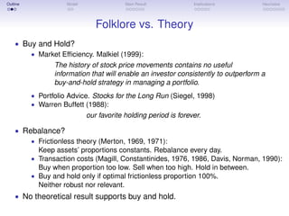
![Outline Model Main Result Implications Heuristics
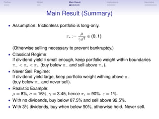
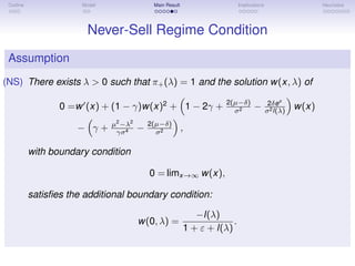
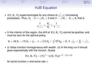
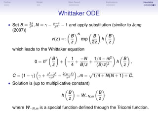
Never Sell. Never Pay Taxes (on Capital Gains).
• Discussion so far neglects effect of taxes on capital gains...
• ...which do not affect the never-sell strategy...
• ...but reduce the performance of other “optimal ” policies...
• ...making never-sell superior after tax.
π∗ [π−, π+] [π−, π+] never sell buy & hold
(average) (specific)
50% 2.41% 2.41% 2.07% 4.48%
60% 2.13% 2.13% 1.83% 3.96%
70% 1.91% 1.91% 1.64% 3.55%
80% 1.49% 1.49% 1.49% 3.22%
90% 1.36% 1.36% 1.36% 2.94%
• Relative loss (EsR0,τ − EsR)/ EsR0,τ with capital gains taxes, for optimal
([π−, π+]), never sell ([π−, 1]), and buy-and-hold ([0, 1]) strategies.
• Simulation with T = 20, time step dt = 1/250, and sample N = 2 × 10⁷
.
• Both taxes on dividends (τ) and capital gains (α) accounted for.
• µ = 8%, σ = 16%, α = 20%, τ = 20%, r = 1%, δ = 2%, and ε = 1%.](https://image.slidesharecdn.com/dividendcork-150826194615-lva1-app6891/85/Who-Should-Sell-Stocks-16-320.jpg)
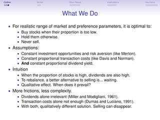
![Outline Model Main Result Implications Heuristics
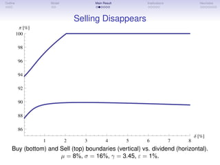
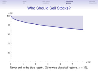
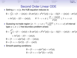
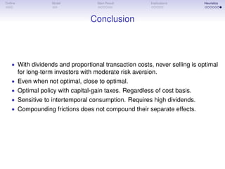
Terms and Conditions
• Never Selling superior to rebalancing for long-term investors with
moderate risk aversion, and no intermediate consumption.
• With high consumption and low dividends selling is necessary.
π∗ [πJS
− , πJS
+ ] never sell buy & hold
50% 1.00% 1.67% 2.00%
60% 0.59% 1.17% 1.47%
70% 0.53% 1.05% 1.05%
80% 0.48% 0.71% 0.71%
90% 0.22% 0.65% 0.65%
• Relative loss (EsR0 − EsR)/ EsR0 of the asymptotically optimal
([πJS
− , πJS
+ ]), never-sell ([π−, 1]) and static buy-and-hold ([0, 1]) strategies
with πJS
± from Janecek-Shreve.
• Simulation with T = 20, time step dt = 1/250, and sample N = 2 × 10⁷
.
• µ = 8%, σ = 16%, ρ = 2%, r = 1%, τ = 0%, ε = 1% and δ = 3%.](https://image.slidesharecdn.com/dividendcork-150826194615-lva1-app6891/85/Who-Should-Sell-Stocks-17-320.jpg)


![[Lehman brothers] interest rate parity, money market basis swaps, and cross c...](https://cdn.slidesharecdn.com/ss_thumbnails/lehmanbrothersinterestrateparitymoneymarketbasisswapsandcross-currencybasisswaps-120814082308-phpapp01-thumbnail.jpg?width=640&height=640&fit=bounds)


![Lecture on nk [compatibility mode]](https://cdn.slidesharecdn.com/ss_thumbnails/lectureonnkcompatibilitymode-110825092241-phpapp01-thumbnail.jpg?width=640&height=640&fit=bounds)


