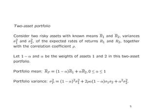
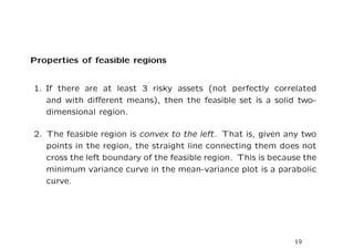
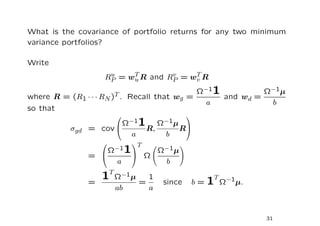
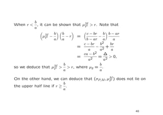
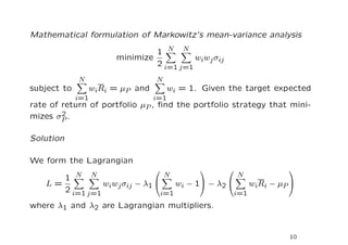
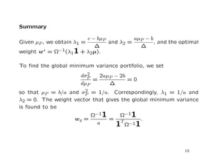
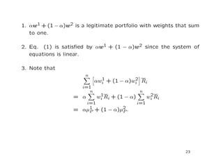
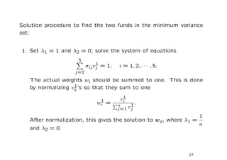
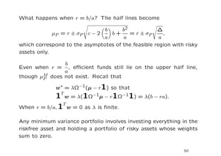
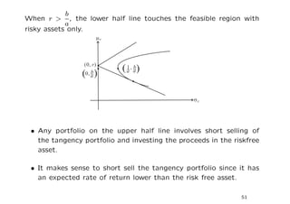
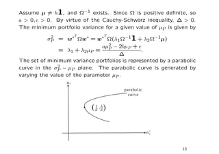
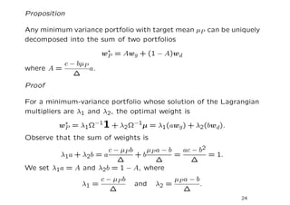
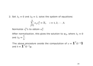
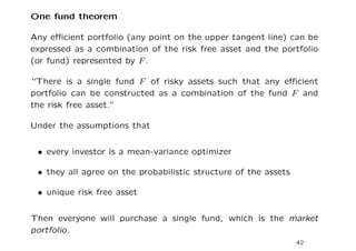
This document summarizes Markowitz's mean-variance portfolio theory and the two-fund theorem. [1] Markowitz formulated the mean-variance model, which minimizes portfolio variance subject to a target expected return. The optimal weights are a function of the covariance matrix and target mean. [2] The two-fund theorem states that any efficient portfolio can be replicated as a combination of two "fundamental" portfolios. Investors only need to invest in these two funds. 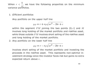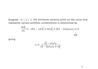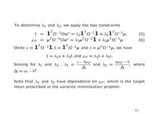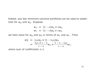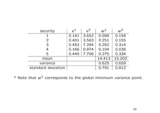[3] The minimum variance set forms the left boundary of the feasible region in mean-variance space. Portfolios on this boundary are efficient funds.

1. 2. Mean-variance portfolio theory
(2.1) Markowitz’s mean-variance formulation
(2.2) Two-fund theorem
(2.3) Inclusion of the riskfree asset
1

2. 2.1 Markowitz mean-variance formulation
Suppose there are N risky assets, whose rates of returns are given by the random
variables R1 , · · · , RN , where
Sn(1) − Sn (0)
Rn = , n = 1, 2, · · · , N.
Sn(0)
Let w = (w1 · · · wN )T , wn denotes the proportion of wealth invested in asset n,
N
with wn = 1. The rate of return of the portfolio is
n=1
N
RP = wnRn .
n=1
Assumptions
1. There does not exist any asset that is a combination of other assets in the
portfolio, that is, non-existence of redundant security.
2. µ = (R1 R2 · · · RN ) and 1
= (1 1 · · · 1) are linearly independent, otherwise
RP is a constant irrespective of any choice of portfolio weights.
2

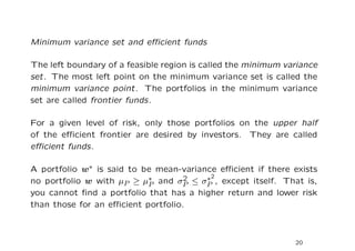
3. The first two moments of RP are
N N
µP = E[RP ] = E[wn Rn] = wnµn, where µn = Rn,
n=1 n=1
and
N N N N
2
σP = var(RP ) = wiwj cov(Ri, Rj ) = wiσij wj .
i=1 j=1 i=1 j=1
Let Ω denote the covariance matrix so that
2
σP = wT Ωw.
For example when n = 2, we have
σ11 σ12 w1 2 2 2 2
(w1 w2 ) = w1 σ1 + w1w2(σ12 + σ21) + w2 σ2 .
σ21 σ22 w2
3

4. Remark
2
1. The portfolio risk of return is quantified by σP . In mean-variance
analysis, only the first two moments are considered in the port-
folio model. Investment theory prior to Markowitz considered
the maximization of µP but without σP .
2. The measure of risk by variance would place equal weight on
the upside deviations and downside deviations.
3. In the mean-variance model, it is assumed that µi, σi and σij are
all known.
4

5. Two-asset portfolio
Consider two risky assets with known means R1 and R2, variances
2 2
σ1 and σ2 , of the expected rates of returns R1 and R2, together
with the correlation coefficient ρ.
Let 1 − α and α be the weights of assets 1 and 2 in this two-asset
portfolio.
Portfolio mean: RP = (1 − α)R1 + αR2, 0 ≤ α ≤ 1
Portfolio variance: σP = (1 − α)2σ1 + 2ρα(1 − α)σ1σ2 + α2σ2 .
2 2 2
5

6. We represent the two assets in a mean-standard deviation diagram
√
(recall: standard deviation = variance)
As α varies, (σP , RP ) traces out a conic curve in the σ − R plane.
With ρ = −1, it is possible to have σ = 0 for some suitable choice of
weight. In general, putting two assets whose returns are negatively
correlated has the desirable effect of lowering the portfolio risk.
6

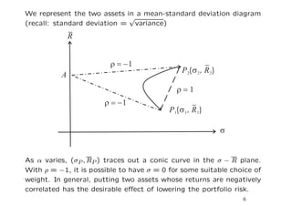
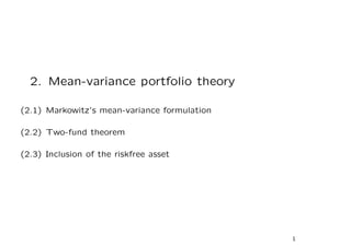
7. In particular, when ρ = 1,
σP (α; ρ = 1) = (1 − α)2σ1 + 2α(1 − α)σ1σ2 + α2σ2
2 2
= (1 − α)σ1 + ασ2.
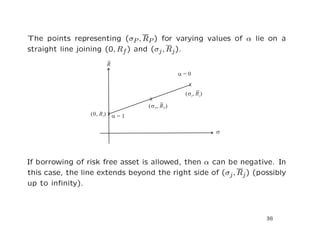
This is the straight line joining P1(σ1, R1) and P2(σ2, R2).
When ρ = −1, we have
σP (α; ρ = −1) = [(1 − α)σ1 − ασ2]2 = |(1 − α)σ1 − ασ2|.
When α is small (close to zero), the corresponding point is close to
P1(σ1, R1). The line AP1 corresponds to
σP (α; ρ = −1) = (1 − α)σ1 − ασ2.
σ1
The point A (with zero σ) corresponds to α = .
σ1 + σ2
σ1
The quantity (1 − α)σ1 − ασ2 remains positive until α = .
σ1 + σ2
σ1
When α > , the locus traces out the upper line AP2.
σ1 + σ2
7

8. Suppose −1 < ρ < 1, the minimum variance point on the curve that
represents various portfolio combinations is determined by
2
∂σP 2 2
= −2(1 − α)σ1 + 2ασ2 + 2(1 − 2α)ρσ1σ2 = 0
∂α
↑
set
giving
2
σ1 − ρσ1σ2
α= 2 2
.
σ1 − 2ρσ1σ2 + σ2
8

9. 9

10. Mathematical formulation of Markowitz’s mean-variance analysis
1 N N
minimize wiwj σij
2 i=1 j=1
N N
subject to wiRi = µP and wi = 1. Given the target expected
i=1 i=1
rate of return of portfolio µP , find the portfolio strategy that mini-
2
mizes σP .
Solution
We form the Lagrangian
   
N N N N
1
L= wiwj σij − λ1  wi − 1 − λ2  wi R i − µ P 
2 i=1 j=1 i=1 i=1
where λ1 and λ2 are Lagrangian multipliers.
10

11. We then differentiate L with respect to wi and the Lagrangian mul-
tipliers, and set the derivative to zero.
N
∂L
= σij wj − λ1 − λ2Ri = 0, i = 1, 2, · · · , N. (1)
∂wi j=1
N
∂L
= wi − 1 = 0; (2)
∂λ1 i=1
N
∂L
= wiRi − µP = 0. (3)
∂λ2 i=1
From Eq. (1), the portfolio weight admits solution of the form
w∗ = Ω−1(λ11 + λ2µ) (4)
where 1 = (1 1 · · · 1)T and µ = (R1 R2 · · · RN )T .
11

12. To determine λ1 and λ2, we apply the two constraints
T T T
1 = 1 Ωw = λ11 Ω 1 + λ21 Ω−1µ.
−1
Ω ∗ −1
(5)
µP = µT Ω−1Ωw∗ = λ1µT Ω−11 + λ2µT Ω−1µ. (6)
T T
Write a = 1 Ω−11, b = 1 Ω−1µ and c = µT Ω−1µ, we have
1 = λ1a + λ2b and µP = λ1b + λ2c.
c − bµP aµP − b
Solving for λ1 and λ2 : λ1 = and λ2 = , where
∆ ∆
∆ = ac − b2.
Note that λ1 and λ2 have dependence on µP , which is the target
mean prescribed in the variance minimization problem.
12

13. Assume µ = h1, and Ω−1 exists. Since Ω is positive definite, so
a > 0, c > 0. By virtue of the Cauchy-Schwarz inequality, ∆ > 0.
The minimum portfolio variance for a given value of µP is given by
∗T ∗T
2
σP = w ∗
Ωw = w Ω(λ1Ω−11 + λ2Ω−1µ)
aµ2 − 2bµP + c
P
= λ1 + λ2µP = .
∆
The set of minimum variance portfolios is represented by a parabolic
2
curve in the σP − µP plane. The parabolic curve is generated by
varying the value of the parameter µP .
13

14. Alternatively, when µP is plotted against σP , the set of minimum
variance portfolio is a hyperbolic curve.
dµP
What are the asymptotic values of lim ?
µ→±∞ dσP
dµP 2
dµP dσP
= 2
dσP dσP dσP
∆
= 2σP
2aµP − 2b
√
∆
= aµ2 − 2bµP + c
P
aµP − b
so that
dµP ∆
lim =± .
µ→±∞ dσP a
14

15. Summary
c − bµP aµP − b
Given µP , we obtain λ1 = and λ2 = , and the optimal
∆ ∆
weight w∗ = Ω−1(λ11 + λ2µ).
To find the global minimum variance portfolio, we set
2
dσP 2aµP − 2b
= =0
dµP ∆
2
so that µP = b/a and σP = 1/a. Correspondingly, λ1 = 1/a and
λ2 = 0. The weight vector that gives the global minimum variance
is found to be
Ω−11 Ω−11
wg = = T
.
a 1 Ω−11
15

16. Another portfolio that corresponds to λ1 = 0 is obtained when µP
c
is taken to be . The value of the other Lagrangian multiplier is
b
given by
a c −b
b 1
λ2 = =
.
∆ b
The weight vector of this particular portfolio is
−1 Ω−1µ
∗ = Ω µ =
wd .
b T
1 Ω−1µ
c 2 − 2b c + c
a b
2 b c
Also, σd = = 2.
∆ b
16

17. Feasible set
Given N risky assets, we form various portfolios from these N assets.
We plot the point (σP , RP ) representing the portfolios in the σ − R
diagram. The collection of these points constitutes the feasible set
or feasible region.
17

18. Consider a 3-asset portfolio, the various combinations of assets 2
and 3 sweep out a curve between them (the particular curve taken
depends on the correlation coefficient ρ12).
A combination of assets 2 and 3 (labelled 4) can be combined with
asset 1 to form a curve joining 1 and 4. As 4 moves between 2 and
3, the curve joining 1 and 4 traces out a solid region.
18

19. Properties of feasible regions
1. If there are at least 3 risky assets (not perfectly correlated
and with different means), then the feasible set is a solid two-
dimensional region.
2. The feasible region is convex to the left. That is, given any two
points in the region, the straight line connecting them does not
cross the left boundary of the feasible region. This is because the
minimum variance curve in the mean-variance plot is a parabolic
curve.
19

20. Minimum variance set and efficient funds
The left boundary of a feasible region is called the minimum variance
set. The most left point on the minimum variance set is called the
minimum variance point. The portfolios in the minimum variance
set are called frontier funds.
For a given level of risk, only those portfolios on the upper half
of the efficient frontier are desired by investors. They are called
efficient funds.
A portfolio w∗ is said to be mean-variance efficient if there exists
2 ∗2
no portfolio w with µP ≥ µ∗ and σP ≤ σP , except itself. That is,
P
you cannot find a portfolio that has a higher return and lower risk
than those for an efficient portfolio.
20

21. 2.2 Two-fund theorem
Two frontier funds (portfolios) can be established so that any fron-
tier portfolio can be duplicated, in terms of mean and variance, as
a combination of these two. In other words, all investors seeking
frontier portfolios need only invest in combinations of these two
funds.
Remark
Any convex combination (that is, weights are non-negative) of ef-
ficient portfolios is an efficient portfolio. Let αi ≥ 0 be the weight
of Fund i whose rate of return is Rfi . Since E Ri ≥ b for all i, we
f a
have
n n
i ≥ b b
αiE Rf αi = .
i=1 i=1 a a
21

22. Proof
Let w1 = (w1 · · · wn ), λ1, λ1 and w2 = (w1 · · · wn )T , λ2, λ2 are two
1 1
1 2
2 2
1 2
known solutions to the minimum variance formulation with expected
rates of return µ1 and µ2 , respectively.
P P
n
σij wj − λ1 − λ2Ri = 0, i = 1, 2, · · · , n (1)
j=1
n
wi r i = µ P (2)
i=1
n
wi = 1. (3)
i=1
It suffices to show that αw1 + (1 − α)w2 is a solution corresponds
to the expected rate of return αµ1 + (1 − α)µ2 .
P P
22

23. 1. αw1 + (1 − α)w2 is a legitimate portfolio with weights that sum
to one.
2. Eq. (1) is satisfied by αw1 + (1 − α)w2 since the system of
equations is linear.
3. Note that
n
1 2
αwi + (1 − α)wi Ri
i=1
n n
1 2
= α wi Ri + (1 − α) wi R i
i=1 i=1
= αµ1 + (1 − α)µ2 .
P P
23

24. Proposition
Any minimum variance portfolio with target mean µP can be uniquely
decomposed into the sum of two portfolios
w∗ = Awg + (1 − A)wd
P
c − bµP
where A = a.
∆
Proof
For a minimum-variance portfolio whose solution of the Lagrangian
multipliers are λ1 and λ2, the optimal weight is
w∗ = λ1Ω−11 + λ2Ω−1µ = λ1(awg ) + λ2(bwd).
P
Observe that the sum of weights is
c − µP b µP a − b ac − b2
λ1a + λ2b = a +b = = 1.
∆ ∆ ∆
We set λ1a = A and λ2b = 1 − A, where
c − µP b µ a−b
λ1 = and λ2 = P .
∆ ∆
24

25. Indeed, any two minimum-variance portfolios can be used to substi-
tute for wg and wd. Suppose
wu = (1 − u)wg + uwd
wv = (1 − v)wg + v wd
we then solve for wg and wd in terms of wu and wv . Then
∗
wP = λ1awg + (1 − λ1a)w d
λ1a + v − 1 1 − u − λ1a
= wu + wv ,
v−u v−u
where sum of coefficients = 1.
25

26. Example
Mean, variances and covariances of the rates of return of 5 risky
assets are listed:
Security covariance Ri
1 2.30 0.93 0.62 0.74 −0.23 15.1
2 0.93 1.40 0.22 0.56 0.26 12.5
3 0.62 0.22 1.80 0.78 −0.27 14.7
4 0.74 0.56 0.78 3.40 −0.56 9.02
5 −0.23 0.26 −0.27 −0.56 2.60 17.68
26

27. Solution procedure to find the two funds in the minimum variance
set:
1. Set λ1 = 1 and λ2 = 0; solve the system of equations
5
1
σij vj = 1, i = 1, 2, · · · , 5.
j=1
The actual weights wi should be summed to one. This is done
1
by normalizing vk ’s so that they sum to one
1
vi
1
wi = n 1
.
j=1 vj
1
After normalization, this gives the solution to wg , where λ1 =
a
and λ2 = 0.
27

28. 2. Set λ1 = 0 and λ2 = 1; solve the system of equations:
5
2
σij vj = Ri, i = 1, 2, · · · , 5.
j=1
2 2
Normalize vi ’s to obtain wi .
After normalization, this gives the solution to wd, where λ1 = 0
1
and λ2 = .
b
The above procedure avoids the computation of a = 1T Ω−11
T
and b = 1 Ω−1µ.
28

29. security v1 v2 w1 w2
1 0.141 3.652 0.088 0.158
2 0.401 3.583 0.251 0.155
3 0.452 7.284 0.282 0.314
4 0.166 0.874 0.104 0.038
5 0.440 7.706 0.275 0.334
mean 14.413 15.202
variance 0.625 0.659
standard deviation 0.791 0.812
* Note that w1 corresponds to the global minimum variance point.
29

30. We know that µg = b/a; how about µd?
T w = µT Ω−1µ c
µd = µ d = .
b b
c b ∆
Difference in expected returns = µd − µg = − = > 0.
b a ab
2 2 c 1 ∆
Also, difference in variances = σd − σg = 2 − = 2 > 0.
b a ab
30

31. What is the covariance of portfolio returns for any two minimum
variance portfolios?
Write
RP = wT R and RP = wT R
u
u
v
v
Ω−11 Ω−1µ
where R = (R1 · · · RN )T . Recall that wg = and wd =
a b
so that
 
σgd = cov 
Ω−1 1 R, Ω−1µ
R
a b
 T
= 
Ω−1 1 Ω
Ω−1µ
a b
=
1T Ω−1µ = 1 since
T
b = 1 Ω−1µ.
ab a
31

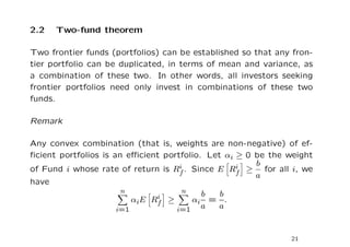
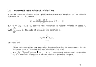
32. In general,
u v 2 2
cov(RP , RP ) = (1 − u)(1 − v)σg + uvσd + [u(1 − v) + v(1 − u)]σgd
(1 − u)(1 − v) uvc u + v − 2uv
= + 2 +
a b a
1 uv∆
= + 2
.
a ab
In particular,
cov(Rg , RP ) = wT ΩwP =
1Ω−1ΩwP 1
= = var(Rg )
g
a a
for any portfolio wP .
For any Portfolio u, we can find another Portfolio v such that these
two portfolios are uncorrelated. This can be done by setting
1 uv∆
+ 2
= 0.
a ab
32

33. The mean-variance criterion can be reconciled with the expected
utility approach in either of two ways: (1) using a quadratic utility
function, or (2) making the assumption that the random returns are
normal variables.
Quadratic utility
b 2
The quadratic utility function can be defined as U (x) = ax − x ,
2
where a > 0 and b > 0. This utility function is really meaningful
only in the range x ≤ a/b, for it is in this range that the function is
increasing. Note also that for b > 0 the function is strictly concave
everywhere and thus exhibits risk aversion.
33

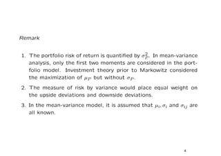
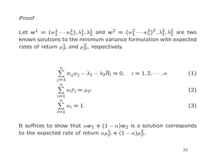
34. mean-variance analysis ⇔ maximum expected utility criterion
based on quadratic utility
Suppose that a portfolio has a random wealth value of y. Using the
expected utility criterion, we evaluate the portfolio using
b 2
E[U (y)] = E ay − y
2
b
= aE[y] − E[y 2]
2
b 2 b
= aE[y] − (E[y]) − var(y).
2 2
Note that we choose the range of the quadratic utility function such
b
that aE[y] − (E[y])2 is increasing in E[y]. Maximizing E[y] for a
2
given var(y) or minimizing var(y) for a given E[y] is equivalent to
maximizing E[U (y)].
34

35. Normal Returns
When all returns are normal random variables, the mean-variance
criterion is also equivalent to the expected utility approach for any
risk-averse utility function.
To deduce this, select a utility function U . Consider a random
wealth variable y that is a normal random variable with mean value
M and standard deviation σ. Since the probability distribution is
completely defined by M and σ, it follows that the expected utility
is a function of M and σ. If U is risk averse, then
∂f ∂f
E[U (y)] = f (M, σ), with >0 and < 0.
∂M ∂σ
35

36. • Now suppose that the returns of all assets are normal random
variables. Then any linear combination of these assets is a nor-
mal random variable. Hence any portfolio problem is therefore
equivalent to the selection of combination of assets that maxi-
mizes the function f (M, σ) with respect to all feasible combina-
tions.
• For a risky-averse utility, this again implies that the variance
should be minimized for any given value of the mean. In other
words, the solution must be mean-variance efficient.
• Portfolio problem is to find w∗ such that f (M, σ) is maximized
with respect to all feasible combinations.
36

37. 2.3 Inclusion of the riskfree asset
Consider a portfolio with weight α for a risk free asset and 1 − α for
a risky asset. The mean of the portfolio is
RP = αRf + (1 − α)Rj (note that Rf = Rf ).
The covariance σf j between the risk free asset and any risky asset
is zero since
E[(Rj − Rj ) (Rf − Rf ) = 0.
zero
2
Therefore, the variance of portfolio σP is
σP = α2 σf +(1 − α)2σj + 2α(1 − α) σf j
2 2 2
zero zero
so that σP = |1 − α|σj .
37

38. The points representing (σP , RP ) for varying values of α lie on a
straight line joining (0, Rf ) and (σj , Rj ).
If borrowing of risk free asset is allowed, then α can be negative. In
this case, the line extends beyond the right side of (σj , Rj ) (possibly
up to infinity).
38

39. Consider a portfolio with N risky assets originally, what is the impact
of the inclusion of a risk free asset on the feasible region?
Lending and borrowing of risk free asset is allowed
For each original portfolio formed using the N risky assets, the new
combinations with the inclusion of the risk free asset trace out the
infinite straight line originating from the risk free point and passing
through the point representing the original portfolio.
The totality of these lines forms an infinite triangular feasible region
bounded by the two tangent lines through the risk free point to the
original feasible region.
39

40. No shorting of the riskfree asset
The line originating from the risk free point cannot be extended
beyond points in the original feasible region (otherwise entail bor-
rowing of the risk free asset). The new feasible region has straight
line front edges.
40

41. The new efficient set is the single straight line on the top of the
new triangular feasible region. This tangent line touches the original
feasible region at a point F , where F lies on the efficient frontier of
the original feasible set.
b
Here, Rf < . This assumption is reasonable since the risk free
a
asset should earn a rate of return less than the expected rate of
return of the global minimum variance portfolio.
41

42. One fund theorem
Any efficient portfolio (any point on the upper tangent line) can be
expressed as a combination of the risk free asset and the portfolio
(or fund) represented by F .
“There is a single fund F of risky assets such that any efficient
portfolio can be constructed as a combination of the fund F and
the risk free asset.”
Under the assumptions that
• every investor is a mean-variance optimizer
• they all agree on the probabilistic structure of the assets
• unique risk free asset
Then everyone will purchase a single fund, which is the market
portfolio.
42

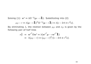
43. Now, the proportion of wealth invested in the risk free asset is
N
1− wi .
i=1
Modified Lagrangian formulation
2
σP 1
minimize = wT Ωw
2 2
subject to wT µ + (1 − wT 1)r = µP .
1 T
Define the Lagrangian: L = w Ωw + λ[µP − r − (µ − r1)T w]
2
N
∂L
= σij wj − λ(µ − r1) = 0, i = 1, 2, · · · , N (1)
∂wi j=1
∂L
=0 giving (µ − r1)T w = µP − r. (2)
∂λ
43

44. Solving (1): w∗ = λΩ−1(µ − r1). Substituting into (2)
µP − r = λ(µ − r1)T Ω−1(µ − r1) = λ(c − 2rb + r2a).
By eliminating λ, the relation between µP and σP is given by the
following pair of half lines
T T T
2
σP = w∗ Ωw∗ = λ(w ∗ µ − rw∗ 1)
= λ(µP − r) = (µP − r)2/(c − 2rb + r2a).
44

45. With the inclusion of the riskfree asset, the set of minimum variance
portfolios are represented by portfolios on the two half lines
Lup : µP − r = σP ar2 − 2br + c (3a)
Llow : µP − r = −σP ar2 − 2br + c. (3b)
Recall that ar2 − 2br + c > 0 for all values of r since ∆ = ac − b2 > 0.
The minimum variance portfolios without the riskfree asset lie on
the hyperbola
2 aµ2 − 2bµP + c
P
σP = .
∆
45

46. b
When r < µg = , the upper half line is a tangent to the hyperbola.
a
The tangency portfolio is the tangent point to the efficient frontier
(upper part of the hyperbolic curve) through the point (0, r).
46

47. The tangency portfolio M is represented by the point (σP,M , µM ),
P
M are obtained by solving simultane-
and the solution to σP,M and µP
ously
2 aµ2 − 2bµP + c
P
σP =
∆
µP = r + σP c − 2rb + r2a.
Once µP is obtained, the corresponding values for λM and w∗ are
M
M
µM − r
λM = P and w∗ = λM Ω−1(µ − r1).
M
c − 2rb + r2a
The tangency portfolio M is shown to be
∗
wM =
Ω−1(µ − r 1) , µM =
c − br
and 2
σP,M =
c − 2rb + r2a
.
P 2
b − ar b − ar (b − ar)
47

48. b
When r < , it can be shown that µM > r. Note that
P
a
M b b c − br b b − ar
µP − −r = −
a a b − ar a a
c − br b2 br
= − 2+
a a a
ca − b2 ∆
= = 2 > 0,
a2 a
M > b > r, where µ = b .
so we deduce that µP g
a a
On the other hand, we can deduce that (σP,M , µM ) does not lie on
P
b
the upper half line if r ≥ .
a
48

49. b
When r < , we have the following properties on the minimum
a
variance portfolios.
1. Efficient portfolios
Any portfolio on the upper half line
µP = r + σP ar2 − 2br + c
within the segment F M joining the two points (0, r) and M
involves long holding of the market portfolio and riskfree asset,
while those outside F M involves short selling of the riskfree asset
and long holding of the market portfolio.
2. Any portfolio on the lower half line
µP = r − σP ar2 − 2br + c
involves short selling of the market portfolio and investing the
proceeds in the riskfree asset. This represents non-optimal in-
vestment strategy since the investor faces risk but gains no extra
expected return above r.
49

50. What happens when r = b/a? The half lines become
b b2 ∆
µP = r ± σP c − 2 b+ = r ± σP ,
a a a
which correspond to the asymptotes of the feasible region with risky
assets only.
b
Even when r = , efficient funds still lie on the upper half line,
a
M does not exist. Recall that
though µP
w∗ = λΩ−1(µ − r1) so that
1T w = λ(1Ω−1µ − r1Ω−11) = λ(b − ra).
T
When r = b/a, 1 w = 0 as λ is finite.
Any minimum variance portfolio involves investing everything in the
riskfree asset and holding a portfolio of risky assets whose weights
sum to zero.
50

51. b
When r > , the lower half line touches the feasible region with
a
risky assets only.
• Any portfolio on the upper half line involves short selling of
the tangency portfolio and investing the proceeds in the riskfree
asset.
• It makes sense to short sell the tangency portfolio since it has
an expected rate of return lower than the risk free asset.
51

52. Interpretation of the tangency portfolio (market portfolio)
• One-fund theorem states that everyone will purchase a single
fund of risky assets and borrow or lend at the risk free rate.
• If everyone purchases the same fund of risky assets, what must
that fund be? This fund must equal the market portfolio.
• The market portfolio is the summation of all assets. If everyone
buys just one fund, and their purchases add up to the market,
then that one fund must be the market as well.
• In the situation where everyone follows the mean-variance method-
ology with the same estimates of parameters, the efficient fund
of risky assets will be the market portfolio.
52

53. How does this happen? The answer is based on the equilibrium
argument.
• If everyone else (or at least a large number of people) solves the
problem, we do not need to. The return on an asset depends
on both its initial price and its final price. The other investors
solve the mean-variance portfolio problem using their common
estimates, and they place orders in the market to acquire their
portfolios.
• If orders placed do not match what is available, the prices must
change. The prices of assets under heavy demand will increase;
the prices of assets under light demand will decrease. These
price changes affect the estimates of asset returns directly, and
hence investors will recalculate their optimal portfolio.
53

54. • This process continues until demand exactly matches supply;
that is, it continues until there is equilibrium.
Summary
• In the idealized world, where every investor is a mean-variance
investor and all have the same estimates, everyone buys the
same portfolio, and that must be equal to the market portfolio.
• Prices adjust to drive the market to efficiency. Then after other
people have made the adjustments, we can be sure that the
efficient portfolio is the market portfolio, so we need not make
any calculations.
54