![Gamma Loss
At time 0, for the delta hedged portfolio,
∂f
π = f(s ) − δ * S and δ = S = S0
0 0 0 ∂S
At time 1,
a) If S moves up to S + Δ S , π 1 = f ( S + Δ S ) − δ * ( S + Δ S )
0 0 0 0
∂f ∂f
Given Negative Gamma, S =S0 + ΔS < S < s< s0 + Δs < δ
∂S ∂S 0
> π − π = f (S + ΔS ) − δ * (S + Δ S ) − f (S ) − δ * S
[ ( ) ]
1 0 0 0 0 0
= f S + ΔS − f (S ) − δ * ΔS
0 0
⎡ ∂f ⎤
= ⎢ S0 <S <S0 +ΔS − δ ⎥ * Δ S = Negative Value * Δ S = Loss;
⎣ ∂S ⎦
b) If S moves down to S − Δ S , π = f (S − ΔS ) − δ * (S − ΔS )
1 0 1 0 0
∂f ∂f
Given Negative Gamma, S =S0 −ΔS > S >S >S0 −ΔS > δ
∂S ∂S 0
> π − π
1 0
[
= f (S − Δ S ) − f (S ) − δ * ΔS
0 0
]
⎡ ∂f ⎤
= ⎢ S 0 > S > S 0 − Δ S − δ ⎥ * ( − Δ S ) = Positive Value * (- Δ S ) = Loss
⎣ ∂S ⎦
11
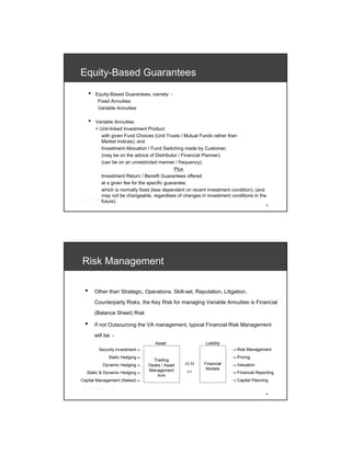
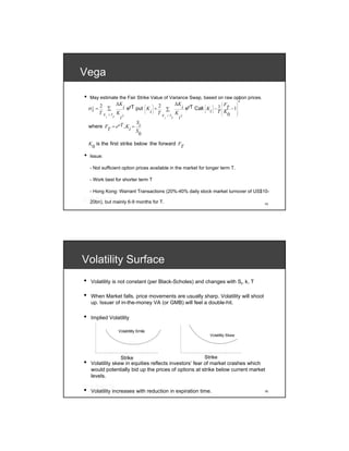
Gamma Loss
• For a Negative Gamma Portfolio, it always loses value on delta re-hedge due to
Buy High / Sell Low phenomenon. It never gains it.
• For each re-hedge, the Loss will equal to ½ * Gamma * (Change of Underlying
Value)2.
• The sum of Gamma Loses, till Expiration, is the actual cost of the option (before
Transaction Costs).
• The cash balance on dynamic hedging a Short Put (negative Г) reduces as
follows: -
1 N −1 2 s −s
= ∑ (r − σ 2Δt ) Γ⎛ ⎞ s 2, where r = i + 1 i ,σ = Implied Volatility
2 i =1 i i ⎜ i, s ⎟ i
⎝ i⎠
i s i
i
← Experienced Volatility < Implied Volatility
← Experienced Volatility = Implied Volatility
12
Option Sold Option Expired](https://image.slidesharecdn.com/soaequitybasedinsuranceguaranteesconference2008-12970889861374-phpapp02/85/Soa-Equity-Based-Insurance-Guarantees-Conference-2008-7-320.jpg)
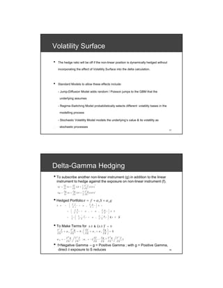
![Delta-Gamma Hedging
• g=Positive Gamma means Long Volatility Option
• Option Illiquid Higher Transaction Costs
• Delta-Gamma Hedging = Dynamic + Static Hedging
• The continuous dynamic hedging (including use of static hedges) will incur
an infinite amount of transaction costs, no matter how small it is.
• In the presence of transaction costs, the absence of arbitrage argument is
invalid, market is incomplete, which leads to many solutions.
• There is no definitive solution on VA management. The success in offering
VA will therefore depend on the availability of the right skill sets, integrated
processes, risk management capabilities by the underwriter to generate
viable and sustained solutions.
19
Hedging Methods
• Finally, the desirable hedging method will, inter alia, depend on Transaction Costs
and the Risk Tolerance / Appetite of the VA underwriter.
• Assume a sale of δ shares of the underlying incurs transaction costs λ/δ/s (λ≥0).
Below are 6 common hedging methods.
a) The Black-Scholes Hedging at Fixed Regular Intervals.
The balance account adjusted on reinstating the target hedge ratio: -
⎡⎛ ∂f ∂f ⎞ ⎛ ∂f ∂f ⎞⎤
⎢⎜ − ⎟ − λ ⎜ − ⎟⎥S
⎜ ⎟ ⎜ ∂S ∂S t ⎟ t+ h
⎢⎝ ∂ S t+
⎣ h ∂S t ⎠ ⎝ t+ h ⎠⎥⎦
b) The Leland Hedging at Fixed Regular Intervals
As per (a) using a modified volatility in the model.
(σ 2
m = σ 2 [1 − λ * Constant * Γ ] )
c) The Delta Tolerance Strategy
∂f
Δ − > h (a given constant) ; Re - hedge to Target Hedge Ratio
∂S
d) The Asset Tolerance Strategy
S (t + Δ t ) − S (t )
> h (a given constant) ; Re - hedge to Target Hedge Ratio
S (t )
20](https://image.slidesharecdn.com/soaequitybasedinsuranceguaranteesconference2008-12970889861374-phpapp02/85/Soa-Equity-Based-Insurance-Guarantees-Conference-2008-11-320.jpg)

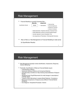
This document discusses quantifying risks associated with equity-based guarantees. It covers: 1) Risk management considerations for variable annuities, including financial modeling to quantify guarantee risks. 2) Basics of dynamic hedging, where the price of an option is the discounted value of dynamically hedging the exposure to expiration. 3) Gamma loss, which occurs when dynamically hedging a negative gamma position, leading to losses from buying high and selling low when re-hedging deltas as the underlying changes value.


