The document discusses a model of dynamic trading volume under price impact. It begins with motivations and an outline of the model, which considers a representative agent facing constant investment opportunities and risk aversion, trading in a market with finite depth. Key results discussed include the optimal trading policy, welfare implications, and dynamics of the implied trading volume. Asymptotic expansions show turnover is proportional to displacement from the target risky weight and depends on parameters like volatility, risk aversion, and market depth. Trading volume is characterized as having properties similar to an Ornstein-Uhlenbeck process. The model provides a way to estimate market depth from observed trading volumes.
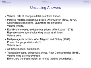

![Model Results Heuristics
Verification
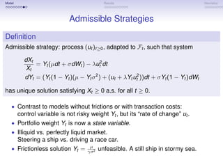
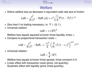
Theorem
µ
If γσ 2
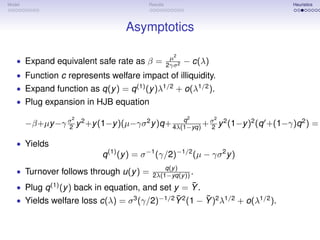
∈ (0, 1), then the optimal wealth turnover and equivalent safe rate are:
1 q(y )
ˆ
u (y ) = ˆ
EsRγ (u ) = β
2λ 1 − yq(y )
2
µ
where β ∈ (0, 2γσ2 ) and q : [0, 1] → R are the unique pair that solves the ODE
2 2 2
q
−β+µy −γ σ y 2 +y (1−y )(µ−γσ 2 y )q+ 4λ(1−yq) + σ y 2 (1−y )2 (q +(1−γ)q 2 ) = 0
2 2
√
and q(0) = 2 λβ, q(1) = λd − λd(λd − 2), where d = −γσ 2 − 2β + 2µ.
• A license to solve an ODE, of Abel type.
• Function q and scalar β not explicit.
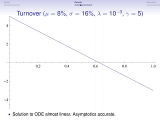
• Asymptotic expansion for λ near zero?](https://image.slidesharecdn.com/quadimpactcolumbia-120611034130-phpapp01/85/Dynamic-Trading-Volume-11-320.jpg)
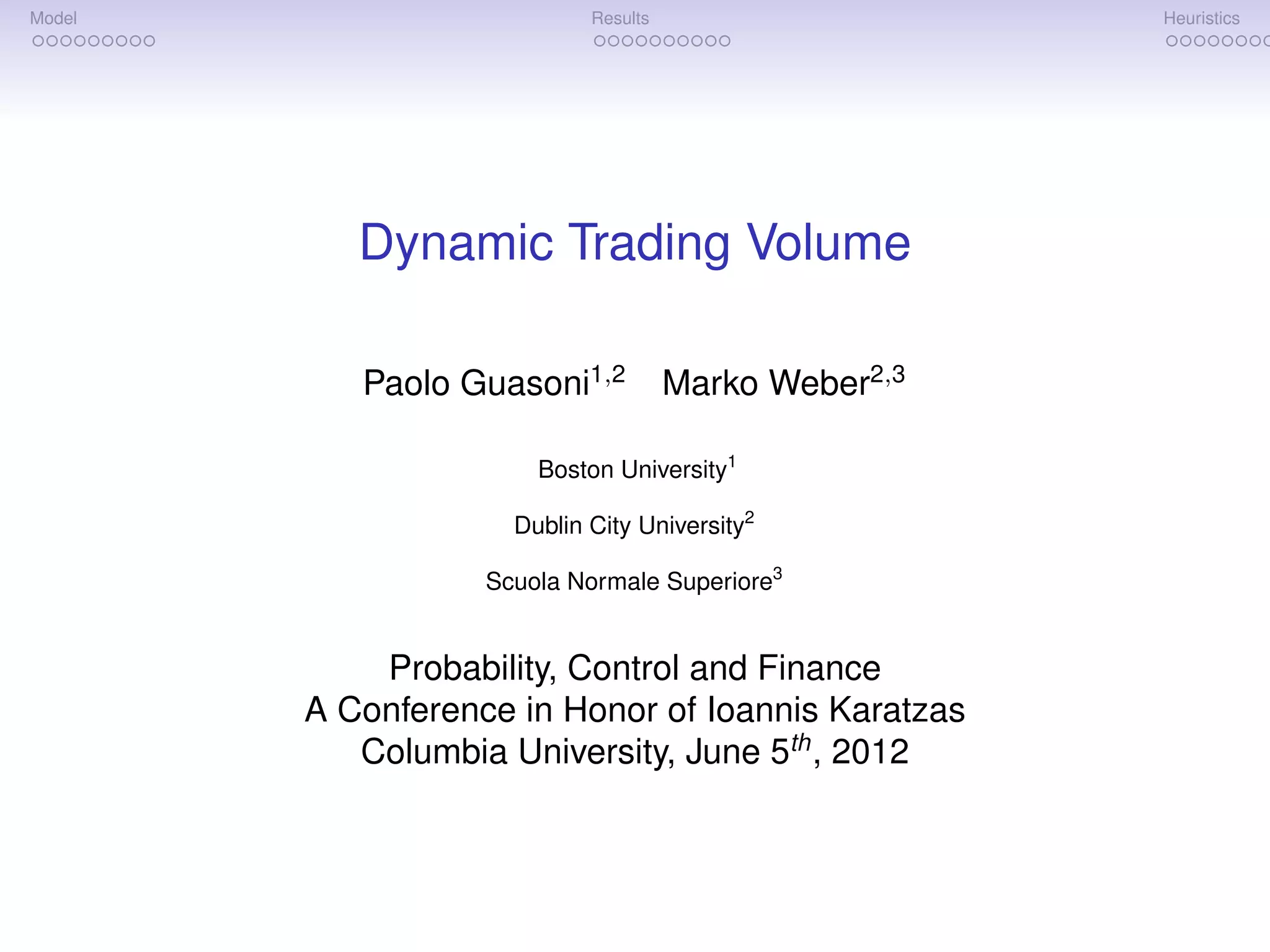
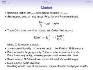
![Model Results Heuristics
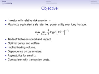
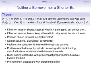
Trading Volume
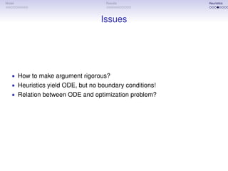
• Wealth turnover approximately Ornstein-Uhlenbeck:
γ 2 ¯2 ¯ γ ¯ ¯
ˆ
d ut = σ (σ Y (1 − Y )(1 − γ) − ut )dt − σ 2
ˆ Y (1 − Y )dWt
2λ 2λ
• In the following sense:
Theorem
ˆ
The process ut has asymptotic moments:
T
1 ¯ ¯
ET := lim u (Yt )dt = σ 2 Y 2 (1 − Y )(1 − γ) + o(1) ,
ˆ
T →∞ T 0
1 T 1 ¯ ¯
VT := lim (u (Yt ) − ET)2 dt = σ 3 Y 2 (1 − Y )2 (γ/2)1/2 λ1/2 + o(λ1/2 ) ,
ˆ
T →∞ T 0 2
1 ¯ ¯
QT := lim E[ u (Y ) T ] = σ 4 Y 2 (1 − Y )2 (γ/2)λ−1 + o(λ−1 )
ˆ
T →∞ T](https://image.slidesharecdn.com/quadimpactcolumbia-120611034130-phpapp01/85/Dynamic-Trading-Volume-17-320.jpg)
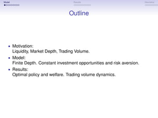
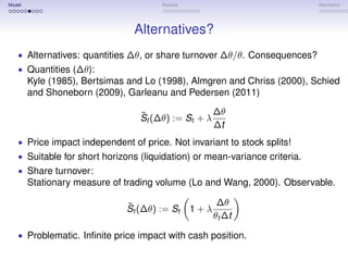
![Model Results Heuristics
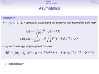
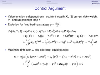
Verification
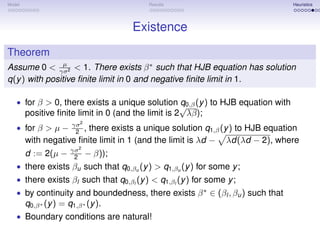
Lemma
y
Let q solve the HJB equation, and define Q(y ) = q(z)dz. There exists a
ˆ
probability P, equivalent to P, such that the terminal wealth XT of any
admissible strategy satisfies:
1−γ 1 1
E[XT ] 1−γ ≤ eβT +Q(y ) EP [e−(1−γ)Q(YT ) ] 1−γ ,
ˆ
and equality holds for the optimal strategy.
• Solution of HJB equation yields asymptotic upper bound for any strategy.
• Upper bound reached for optimal strategy.
• Valid for any β, for corresponding Q.
• Idea: pick largest β ∗ to make Q disappear in the long run.
• A priori bounds:
µ2
β∗ < (frictionless solution)
2γσ 2
γ 2
max 0, µ − σ <β ∗ (all in safe or risky asset)
2](https://image.slidesharecdn.com/quadimpactcolumbia-120611034130-phpapp01/85/Dynamic-Trading-Volume-25-320.jpg)


![[Lehman brothers] interest rate parity, money market basis swaps, and cross c...](https://cdn.slidesharecdn.com/ss_thumbnails/lehmanbrothersinterestrateparitymoneymarketbasisswapsandcross-currencybasisswaps-120814082308-phpapp01-thumbnail.jpg?width=640&height=640&fit=bounds)


