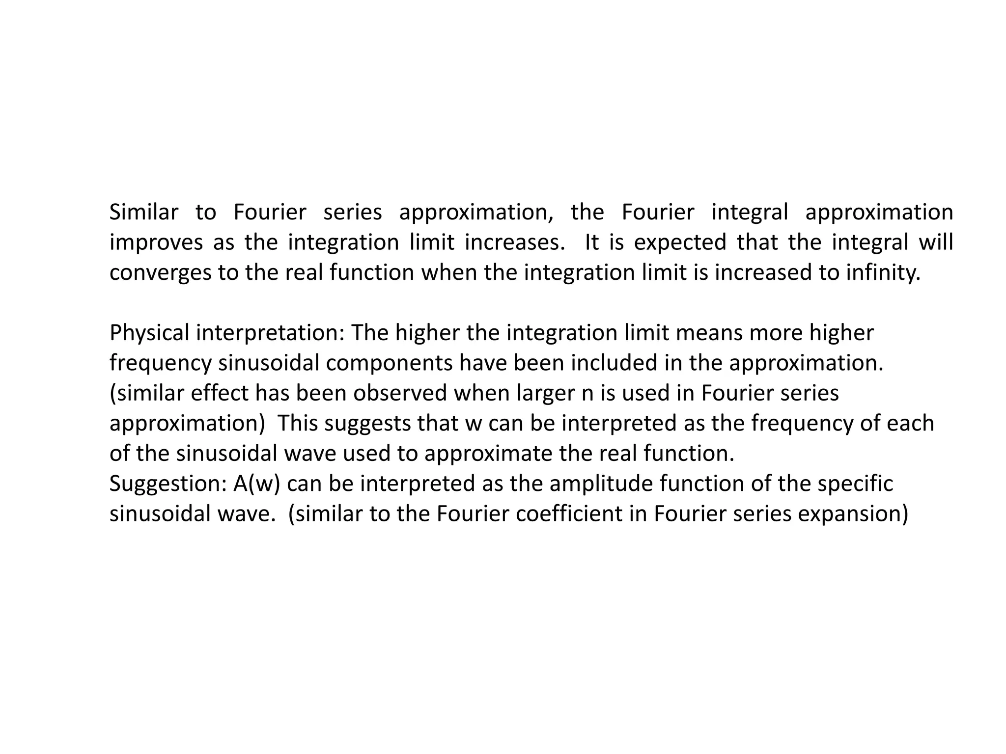
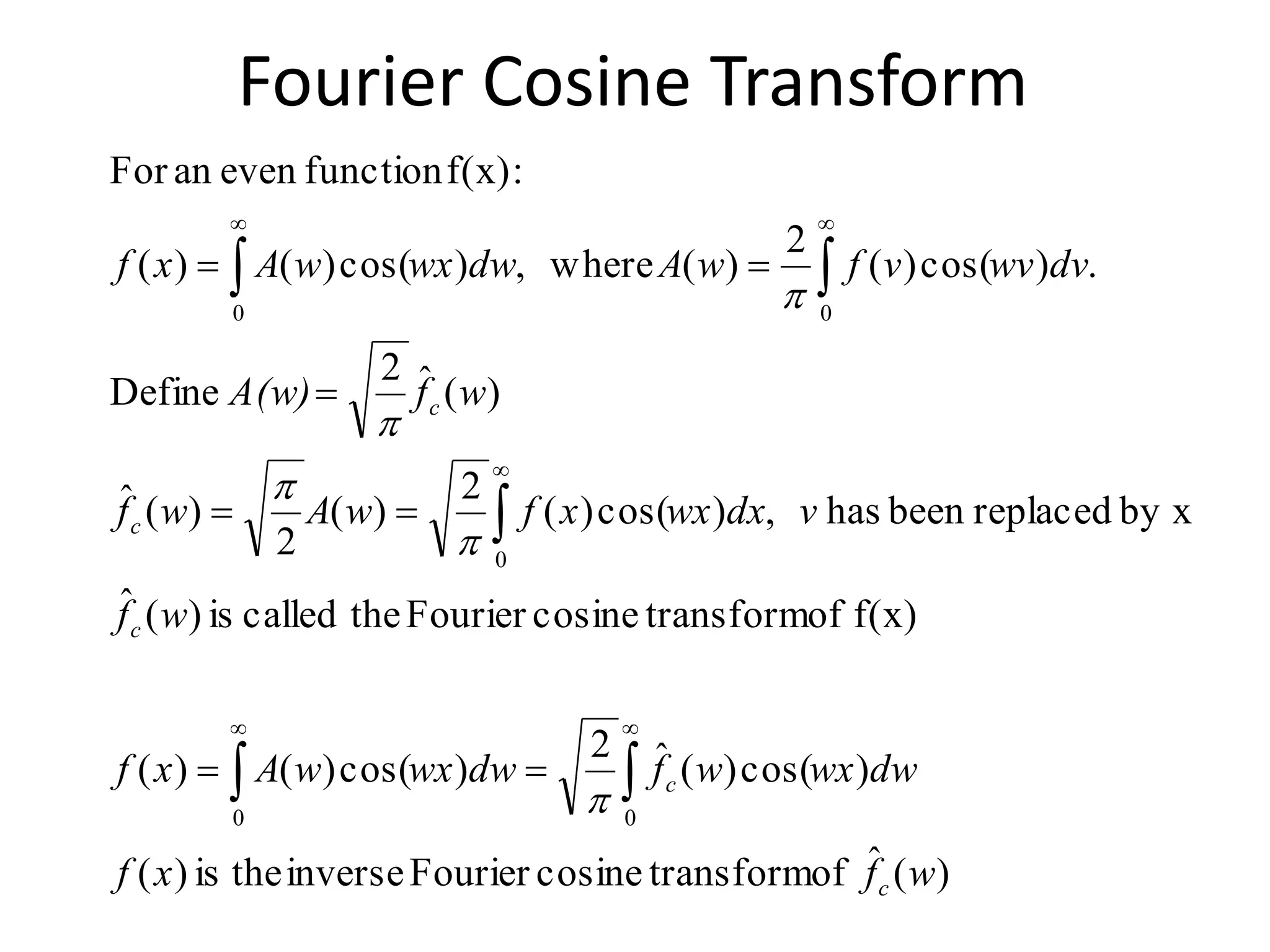
This document discusses Fourier cosine and sine integrals. It provides the definitions and formulas for the Fourier cosine transform, Fourier sine transform, and their inverses. It also discusses improper integrals of type 1 and 2, including definitions and convergence conditions. Examples are provided to illustrate the concepts. The physical interpretation of the Fourier integrals is that higher integration limits include more higher frequency sinusoidal components in the approximation of the real function.

1. UNIT - II

2. Fourier Cosine & Sine Integrals
IntegralSineFourier:)sin()()(,0)(
)sin()(
1
oddisf(x)functiontheIf
IntegralCosineFourier:)cos()()(
0)(
)cos()(
2
)(
1
)(
1
)cos()(
1
A(w)evenisf(x)functiontheIf
0
0
00
0



















dwwxwBxfwA
dvwvvfB(w)
dwwxwAxf
wB
dvwvvfdvdv
dvwvvf




3. Example
dwwx
w
w
dwwxwAf(x)
dvwvdvwvvfwB
w
w
dvwvdvwvvfwA
f(x)
)cos(
)sin(2
)cos()(
isfofintegralFourierThe
0)sin(
1
)sin()(
1
)(
)sin(2
)cos(
1
)cos()(
1
)(
1xfor0
1x1-for1
Let
00
1
1
1
1
1
1





















4. 2 1 0 1 2
0
1
1.5
0.5
f 10 x( )
f 100 x( )
g x( )
22 x
f10 integrate from 0 to 10
f100 integrate from 0 to 100
g(x) the real function

5. Similar to Fourier series approximation, the Fourier integral approximation
improves as the integration limit increases. It is expected that the integral will
converges to the real function when the integration limit is increased to infinity.
Physical interpretation: The higher the integration limit means more higher
frequency sinusoidal components have been included in the approximation.
(similar effect has been observed when larger n is used in Fourier series
approximation) This suggests that w can be interpreted as the frequency of each
of the sinusoidal wave used to approximate the real function.
Suggestion: A(w) can be interpreted as the amplitude function of the specific
sinusoidal wave. (similar to the Fourier coefficient in Fourier series expansion)

6. Fourier Cosine Transform
)(ˆoftransformcosineFourierinversetheis)(
)cos()(ˆ2
)cos()()(
f(x)oftransformcosineFourierthecalledis)(ˆ
by xreplacedbeenhas,)cos()(
2
)(
2
)(ˆ
)(ˆ2
Define
.)cos()(
2
)(where,)cos()()(
:f(x)functionevenanFor
00
0
00
wfxf
dwwxwfdwwxwAxf
wf
vdxwxxfwAwf
wfA(w)
dvwvvfwAdwwxwAxf
c
c
c
c
c
















7. Fourier Sine Transform
)(ˆoftransformsineFourierinversetheis)(
)sin()(ˆ2
)sin()()(
f(x)oftransformsineFourierthecalledis)(ˆ
by xreplacedbeenhas,)sin()(
2
)(
2
)(ˆ
)(ˆ2
Define
.)sin()(
2
)(where,)sin()()(
:f(x)functionoddanforSimilarly,
00
0
00
wfxf
dwwxwfdwwxwBxf
wf
vdxwxxfwBwf
wfB(w)
dvwvvfwBdwwxwBxf
S
S
S
S
S
















8. Improper Integral of Type 1
a) If exists for every number t ≥ a, then
provided this limit exists (as a finite number).
b) If exists for every number t ≤ b, then
provided this limit exists (as a finite number).
The improper integrals and are called
convergent if the corresponding limit exists and divergent
if the limit does not exist.
c) If both and are convergent, then we
define

t
a
dxxf )(

b
t
dxxf )(




t
aa
t
dxxfdxxf )()( lim



b
t
b
t
dxxfdxxf )()( lim


a
dxxf )( 
a
dxxf )(


a
dxxf )(  
b
dxxf )(






a
a
dxxfdxxfdxxf )()()(

9. Examples
1
1
11111
.1 limlimlim 1
1 21 2











 tx
dx
x
dx
x t
t
t
t
t
    1.2 0000
limlimlim 

 
t
t
t
x
t
t
x
t
x
eeedxedxe
   
    
























  
22
tantan
tantan
1
1
1
1
1
1
.3
11
0
101
0
0 222
limlim
limlim
tt
xx
dx
x
dx
x
dx
x
tt
t
t
t
t
All three integrals are convergent.

10.     


 1lnlnln
11
limlimlim 111
txdx
x
dx
x t
t
t
t
t
An example of a divergent integral:
The general rule is the following:
1pifdivergentand1pifconvergentis
1
1


dx
xp


1 2
convergentis
1
thatslidepreviousthefromRecall dx
x

11. Definition of an Improper Integral of Type 2
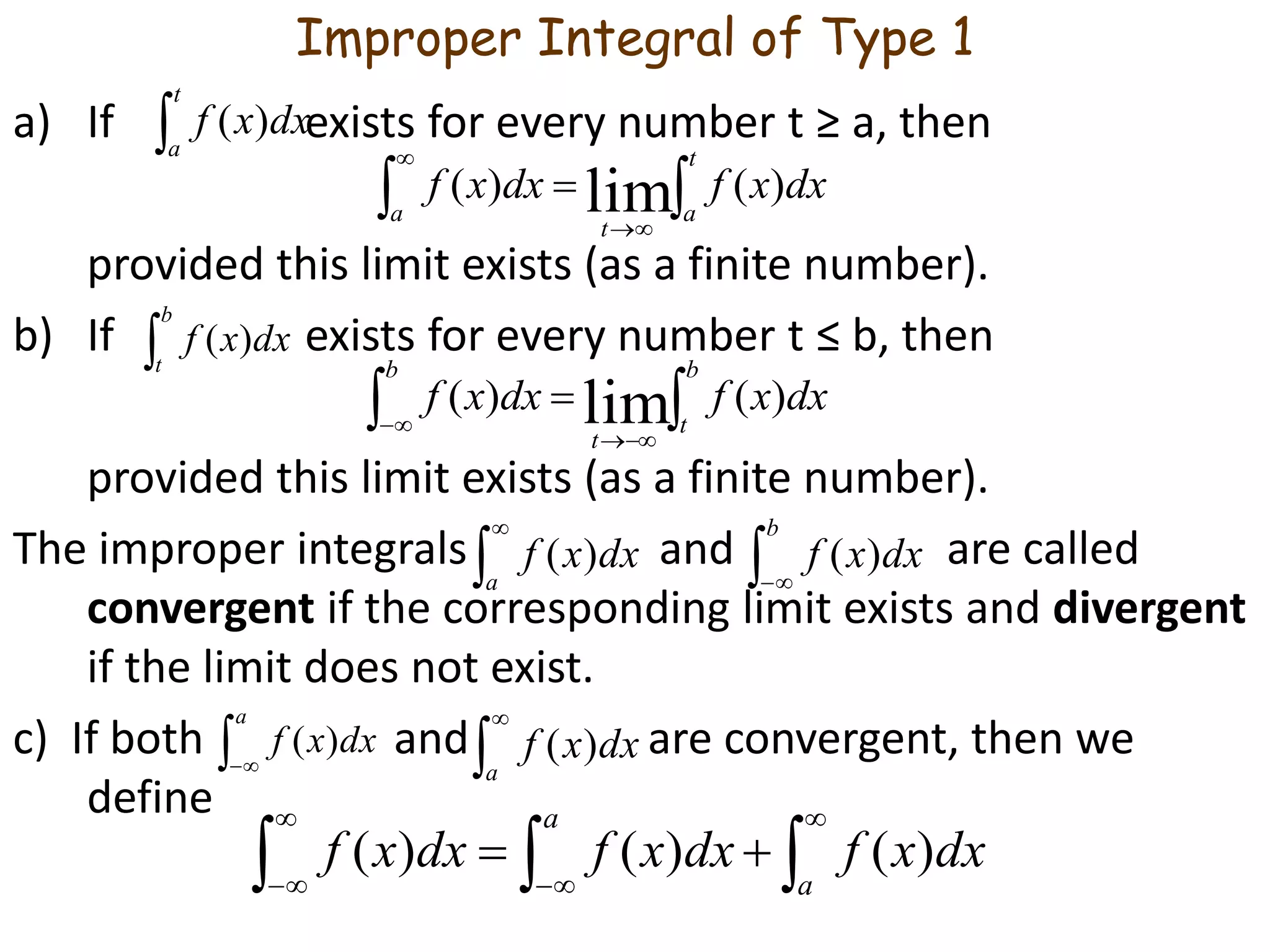
a) If f is continuous on [a, b) and is discontinuous at b, then
if this limit exists (as a finite number).
a) If f is continuous on (a, b] and is discontinuous at a, then
if this limit exists (as a finite number).
The improper integral is called convergent if the
corresponding limit exists and divergent if the limit does
not exist.
c) If f has a discontinuity at c, where a < c < b, and both
and are convergent, then we define
 


t
a
b
a
bt
dxxfdxxf )()( lim
 


b
t
b
a
at
dxxfdxxf )()( lim

b
c
dxxf )(
c
a
dxxf )(

b
a
dxxf )(
 
b
c
c
a
b
a
dxxfdxxfdxxf )()()(