unit commit lecture 2

1. Unit Commitment
Baosen Zhang

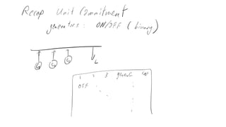
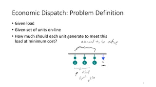
3. Economic Dispatch: Problem Definition
2
• Given load
• Given set of units on-line
• How much should each unit generate to meet this
load at minimum cost?
A B C
L

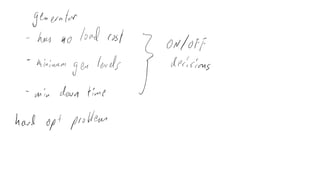
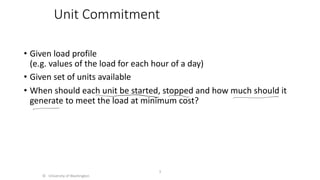
4. Unit Commitment
• Given load profile
(e.g. values of the load for each hour of a day)
• Given set of units available
• When should each unit be started, stopped and how much should it
generate to meet the load at minimum cost?
© University of Washington
3

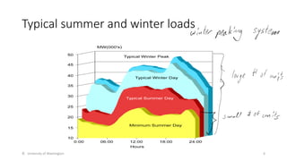
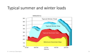
5. Typical summer and winter loads
© University of Washington 4

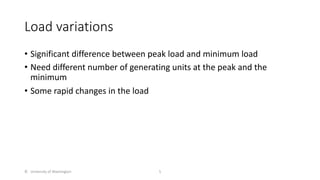
6. Load variations
• Significant difference between peak load and minimum load
• Need different number of generating units at the peak and the
minimum
• Some rapid changes in the load
© University of Washington 5

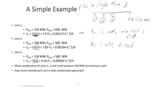
7. A Simple Example
• Unit 1:
• PMin = 250 MW, PMax = 600 MW
• C1 = 510.0 + 7.9 P1 + 0.00172 P1
2 $/h
• Unit 2:
• PMin = 200 MW, PMax = 400 MW
• C2 = 310.0 + 7.85 P2 + 0.00194 P2
2 $/h
• Unit 3:
• PMin = 150 MW, PMax = 500 MW
• C3 = 78.0 + 9.56 P3 + 0.00694 P3
2 $/h
• What combination of units 1, 2 and 3 will produce 550 MW at minimum cost?
• How much should each unit in that combination generate?
© University of Washington
6

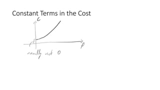
8. Constant Terms in the Cost

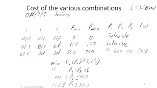
9. Cost of the various combinations
© University of Washington
8

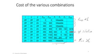
10. Cost of the various combinations
© University of Washington
9
1 2 3 Pmin Pmax P1 P2 P3 Ctotal
Off Off Off 0 0 Infeasible
Off Off On 150 500 Infeasible
Off On Off 200 400 Infeasible
Off On On 350 900 0 400 150 5418
On Off Off 250 600 550 0 0 5389
On Off On 400 1100 400 0 150 5613
On On Off 450 1000 295 255 0 5471
On On On 600 1500 Infeasible -

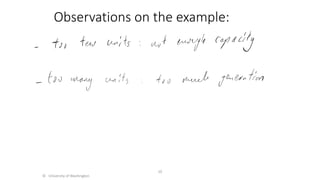
11. Observations on the example:
© University of Washington
10

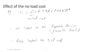
12. Effect of the no-load cost
© University of Washington 11

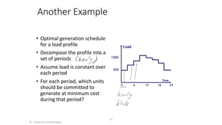
13. Another Example
• Optimal generation schedule
for a load profile
• Decompose the profile into a
set of periods
• Assume load is constant over
each period
• For each period, which units
should be committed to
generate at minimum cost
during that period?
© University of Washington
12
Load
Time
12
6
0 18 24
500
1000

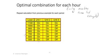
14. Optimal combination for each hour
Load Unit 1 Unit 2 Unit 3
1100 On On On
1000 On On Off
900 On On Off
800 On On Off
700 On On Off
600 On Off Off
500 On Off Off
© University of Washington
13
Repeat calculation from previous example for each period

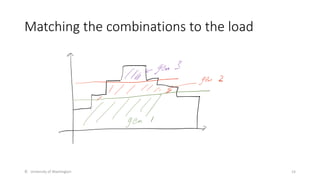
15. Matching the combinations to the load
© University of Washington 14

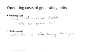
16. Operating costs of generating units
• Running cost
• Start-up cost
© University of Washington
15

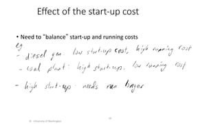
17. Effect of the start-up cost
• Need to “balance” start-up and running costs
© University of Washington
16

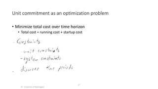
18. Unit commitment as an optimization problem
• Minimize total cost over time horizon
• Total cost = running cost + startup cost
© University of Washington
17

19. Notations
© University of Washington 18

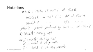
20. Notations
© University of Washington 19
u(i,t): Status of unit i at period t
p(i,t): Power produced by unit i during period t
Unit i is ON during period t
u(i,t) = 1:
Unit i is OFF during period t
u(i,t) = 0 :
Ci[p(i,t)]: Running cost of unit i during period t
SCi[u(i,t)]: Startup cost of unit i during period t
N : Number of available generating units
T : Number of periods in the optimization horizon

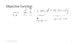
21. Objective function
© University of Washington 20

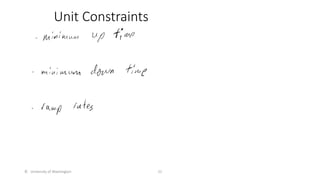
22. Unit Constraints
© University of Washington 21

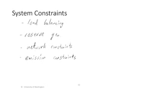
23. System Constraints
© University of Washington
22

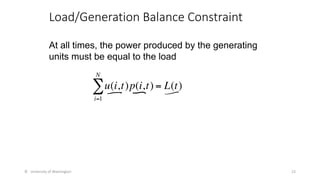
24. Load/Generation Balance Constraint
© University of Washington 23
u(i,t)p(i,t)
i=1
N
∑ = L(t)
At all times, the power produced by the generating
units must be equal to the load

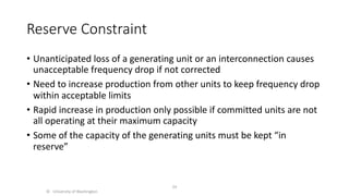
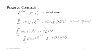
25. Reserve Constraint
• Unanticipated loss of a generating unit or an interconnection causes
unacceptable frequency drop if not corrected
• Need to increase production from other units to keep frequency drop
within acceptable limits
• Rapid increase in production only possible if committed units are not
all operating at their maximum capacity
• Some of the capacity of the generating units must be kept “in
reserve”
© University of Washington
24

26. Reserve Constraint
© University of Washington 25

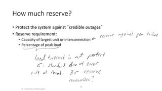
27. How much reserve?
• Protect the system against “credible outages”
• Reserve requirement:
• Capacity of largest unit or interconnection
• Percentage of peak load
© University of Washington
26

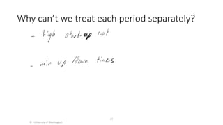
28. Why can’t we treat each period separately?
© University of Washington
27

29. Typical summer and winter loads
© University of Washington 28

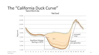
30. The “California Duck Curve”
© 2011 D. Kirschen and University of
Washington
29
Typical March day

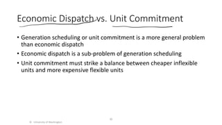
31. Economic Dispatch vs. Unit Commitment
• Generation scheduling or unit commitment is a more general problem
than economic dispatch
• Economic dispatch is a sub-problem of generation scheduling
• Unit commitment must strike a balance between cheaper inflexible
units and more expensive flexible units
© University of Washington
30

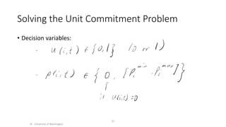
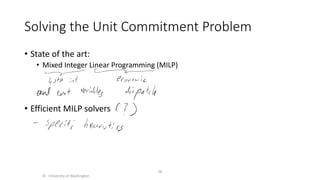
32. Solving the Unit Commitment Problem
• Decision variables:
© University of Washington
31

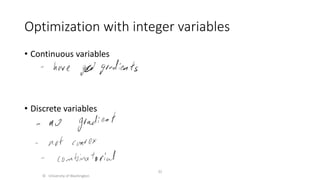
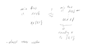
33. Optimization with integer variables
• Continuous variables
• Discrete variables
© University of Washington
32

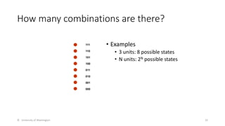
34. How many combinations are there?
© University of Washington 33
• Examples
• 3 units: 8 possible states
• N units: 2N possible states
111
110
101
100
011
010
001
000

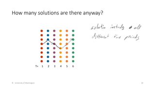
35. How many solutions are there anyway?
© University of Washington 34
1 2 3 4 5 6
T=

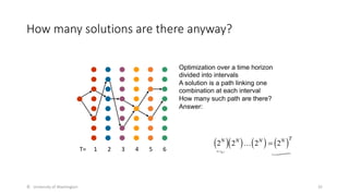
36. How many solutions are there anyway?
© University of Washington 35
1 2 3 4 5 6
T=
Optimization over a time horizon
divided into intervals
A solution is a path linking one
combination at each interval
How many such path are there?
Answer:
2N
( ) 2N
( )… 2N
( ) = 2N
( )T

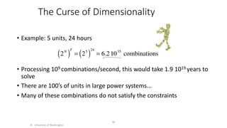
37. The Curse of Dimensionality
• Example: 5 units, 24 hours
• Processing 109 combinations/second, this would take 1.9 1019 years to
solve
• There are 100’s of units in large power systems...
• Many of these combinations do not satisfy the constraints
© University of Washington
36
2N
( )
T
= 25
( )
24
= 6.21035
combinations

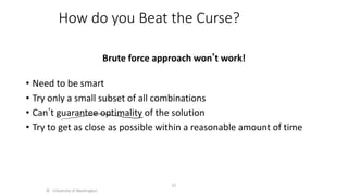
38. How do you Beat the Curse?
Brute force approach wonʼt work!
• Need to be smart
• Try only a small subset of all combinations
• Canʼt guarantee optimality of the solution
• Try to get as close as possible within a reasonable amount of time
© University of Washington
37

40. Solving the Unit Commitment Problem
• State of the art:
• Mixed Integer Linear Programming (MILP)
• Efficient MILP solvers
© University of Washington
38

42. A Simple Unit Commitment Example

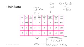
43. Unit Data
© University of Washington 40
Unit
Pmin
(MW)
Pmax
(MW)
Min
up
(h)
Min
down
(h)
No-load
cost
($)
Marginal
cost
($/MWh)
Start-up
cost
($)
Initial
status
A 150 250 3 3 0 10 1,000 ON
B 50 100 2 1 0 12 600 OFF
C 10 50 1 1 0 20 100 OFF

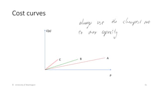
44. Cost curves
© University of Washington 41
p
C(p)
A
B
C

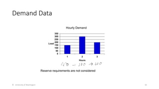
45. Demand Data
© University of Washington 42
Hourly Demand
0
50
100
150
200
250
300
350
1 2 3
Hours
Load
Reserve requirements are not considered

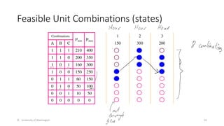
46. Feasible Unit Combinations (states)
© University of Washington 43
Combinations
Pmin Pmax
A B C
1 1 1 210 400
1 1 0 200 350
1 0 1 160 300
1 0 0 150 250
0 1 1 60 150
0 1 0 50 100
0 0 1 10 50
0 0 0 0 0
1 2 3
150 300 200

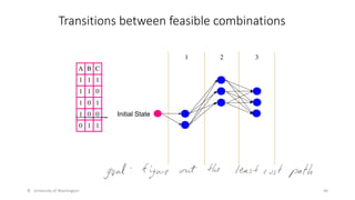
47. Transitions between feasible combinations
© University of Washington 44
A B C
1 1 1
1 1 0
1 0 1
1 0 0
0 1 1
1 2 3
Initial State

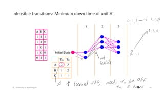
48. Infeasible transitions: Minimum down time of unit A
© University of Washington 45
A B C
1 1 1
1 1 0
1 0 1
1 0 0
0 1 1
1 2 3
Initial State
TD TU
A 3 3
B 1 2
C 1 1

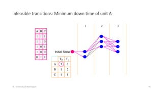
49. Infeasible transitions: Minimum down time of unit A
© University of Washington 46
A B C
1 1 1
1 1 0
1 0 1
1 0 0
0 1 1
1 2 3
Initial State
TD TU
A 3 3
B 1 2
C 1 1

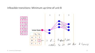
50. Infeasible transitions: Minimum up time of unit B
© University of Washington 47
A B C
1 1 1
1 1 0
1 0 1
1 0 0
0 1 1
1 2 3
Initial State
TD TU
A 3 3
B 1 2
C 1 1

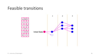
51. Feasible transitions
© University of Washington 48
A B C
1 1 1
1 1 0
1 0 1
1 0 0
0 1 1
1 2 3
Initial State

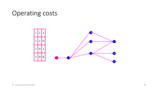
52. Operating costs
© University of Washington 49
1 1 1
1 1 0
1 0 1
1 0 0 1
4
3
2
5
6
7

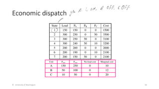
53. Economic dispatch
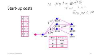
© University of Washington 50
State Load PA PB PC Cost
1 150 150 0 0 1500
2 300 250 0 50 3500
3 300 250 50 0 3100
4 300 240 50 10 3200
5 200 200 0 0 2000
6 200 190 0 10 2100
7 200 150 50 0 2100
Unit Pmin Pmax No-load cost Marginal cost
A 150 250 0 10
B 50 100 0 12
C 10 50 0 20

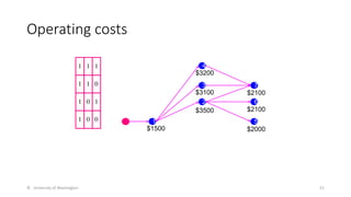
54. Operating costs
© University of Washington 51
1 1 1
1 1 0
1 0 1
1 0 0 1
4
3
2
5
6
7
$1500
$3500
$3100
$3200
$2000
$2100
$2100

55. Start-up costs
© University of Washington 52
1 1 1
1 1 0
1 0 1
1 0 0 1
4
3
2
5
6
7
$1500
$3500
$3100
$3200
$2000
$2100
$2100
Unit Start-up cost
A 1000
B 600
C 100

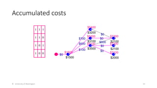
56. Accumulated costs
© University of Washington 53
1 1 1
1 1 0
1 0 1
1 0 0 1
4
3
2
5
6
7
$1500
$3500
$3100
$3200
$2000
$2100
$2100
$1500
$5100
$5200
$5400
$7300
$7200
$7100
$0
$0
$0
$0
$0
$600
$100
$600
$700

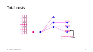
57. Total costs
© University of Washington 54
1 1 1
1 1 0
1 0 1
1 0 0 1
4
3
2
5
6
7
$7300
$7200
$7100
Lowest total cost

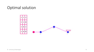
58. Optimal solution
© University of Washington 55
1 1 1
1 1 0
1 0 1
1 0 0 1
2
5
$7100

59. Notes
• This example is intended to illustrate the principles of unit
commitment
• Some constraints have been ignored and others artificially tightened
to simplify the problem and make it solvable by hand
• Therefore it does not illustrate the true complexity of the problem
• The solution method used in this example is based on dynamic
programming. This technique is no longer used in industry because it
only works for small systems (< 20 units)
© University of Washington
56