Download to read offline

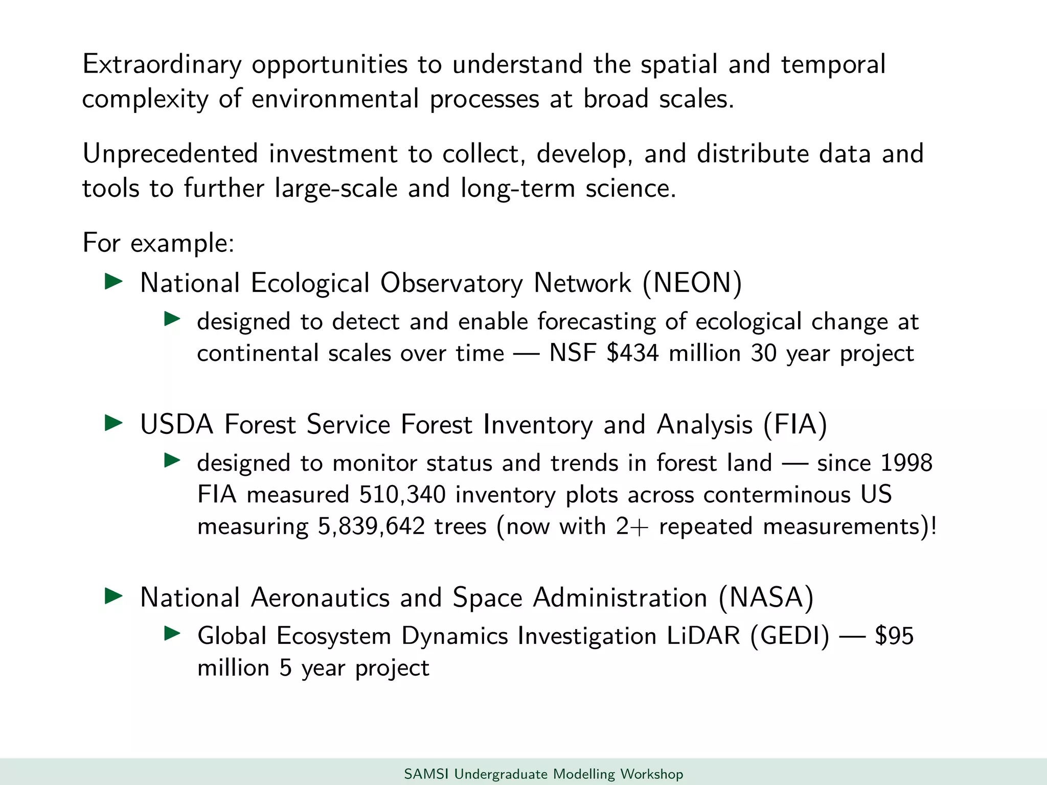
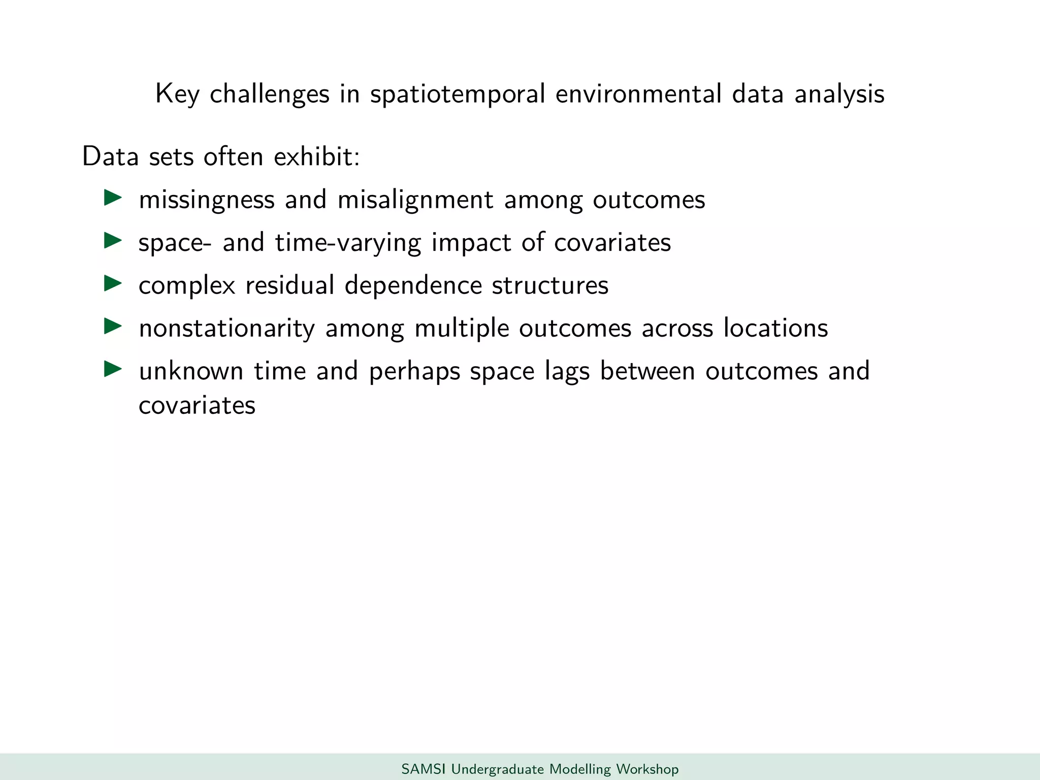
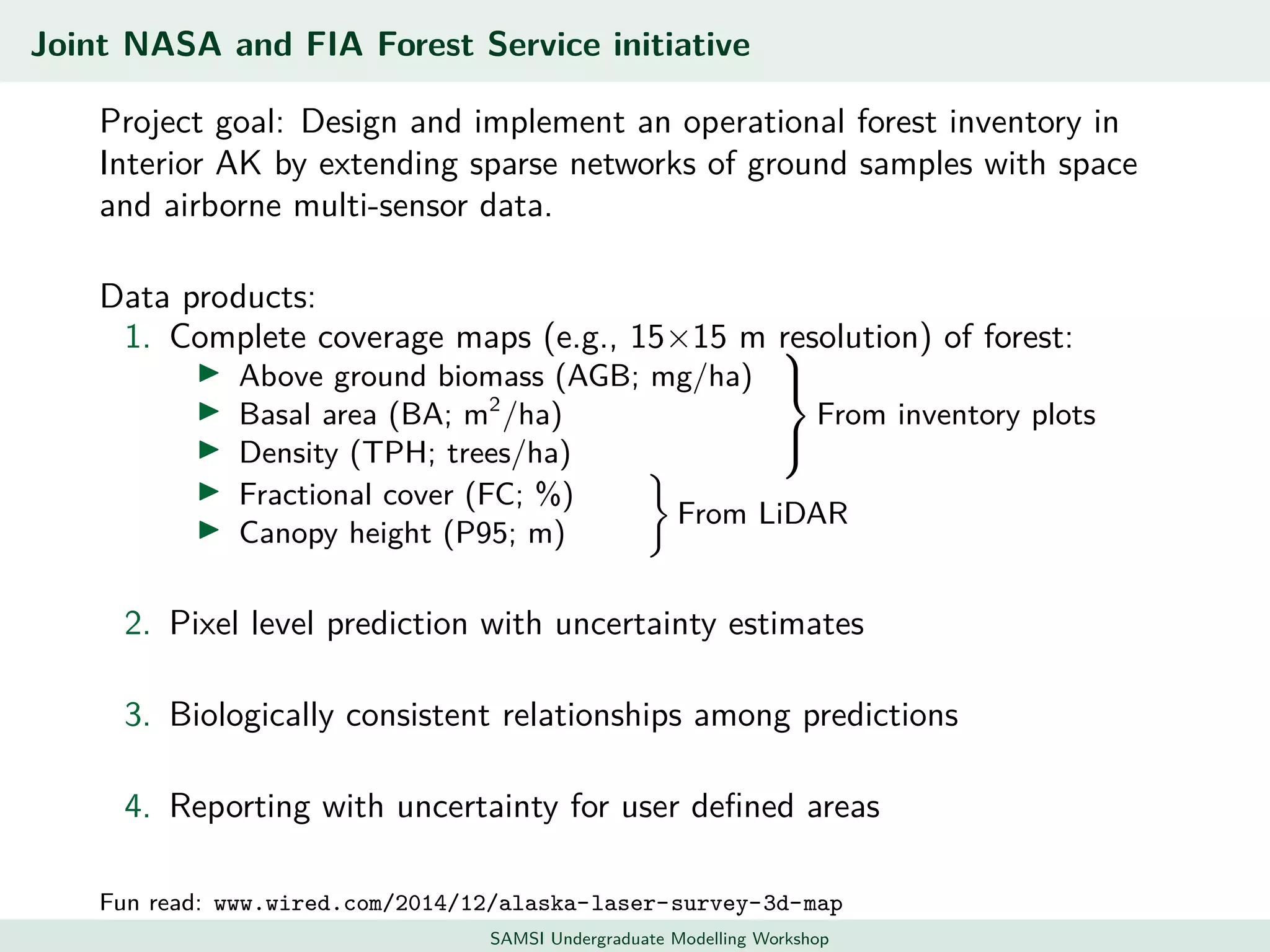
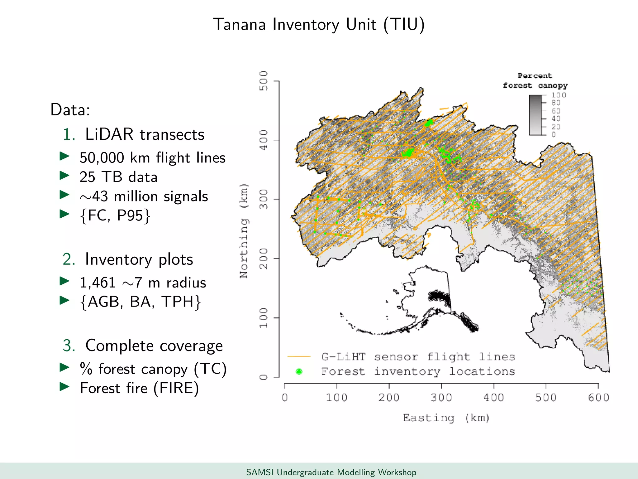
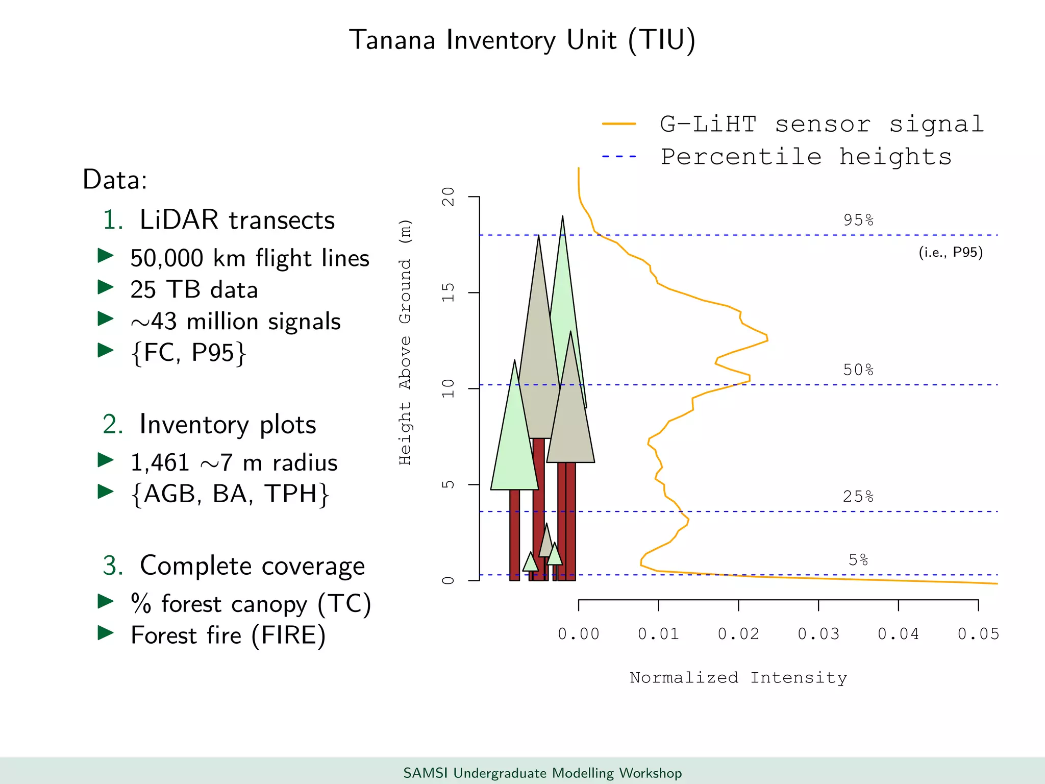

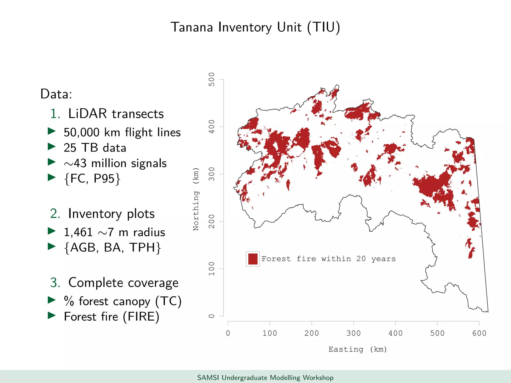
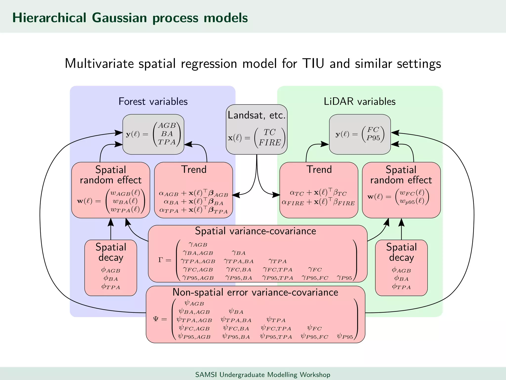
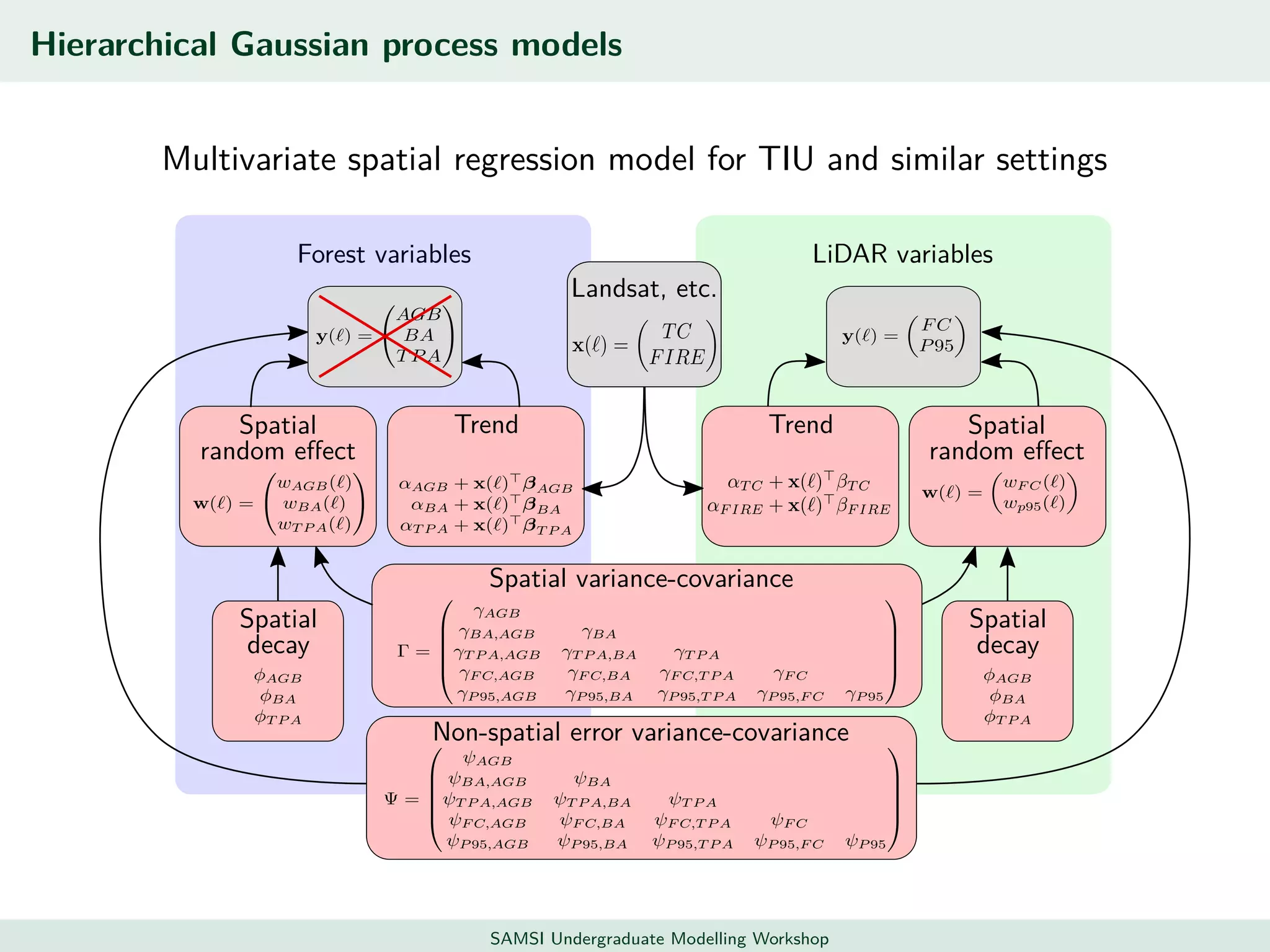
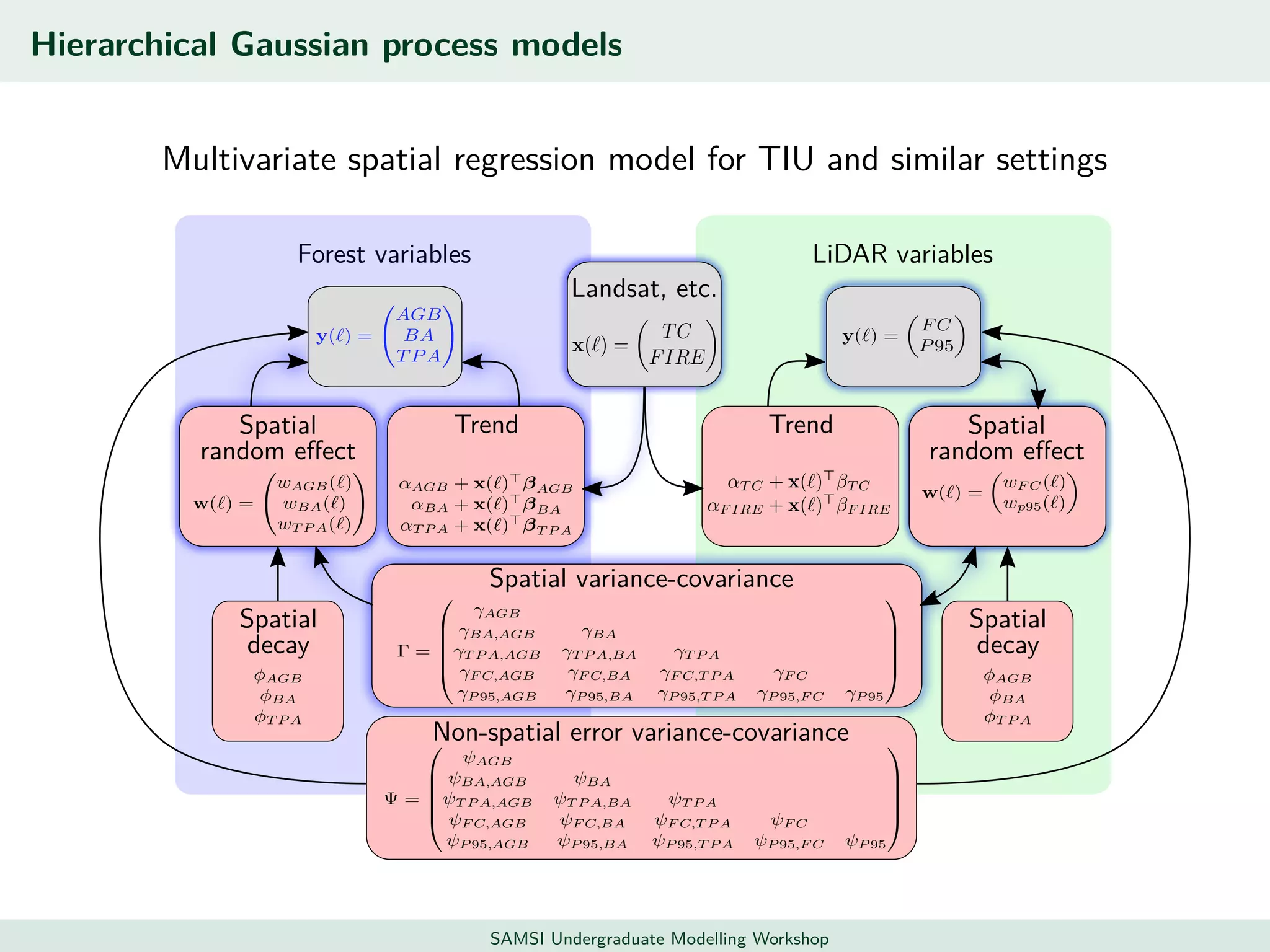
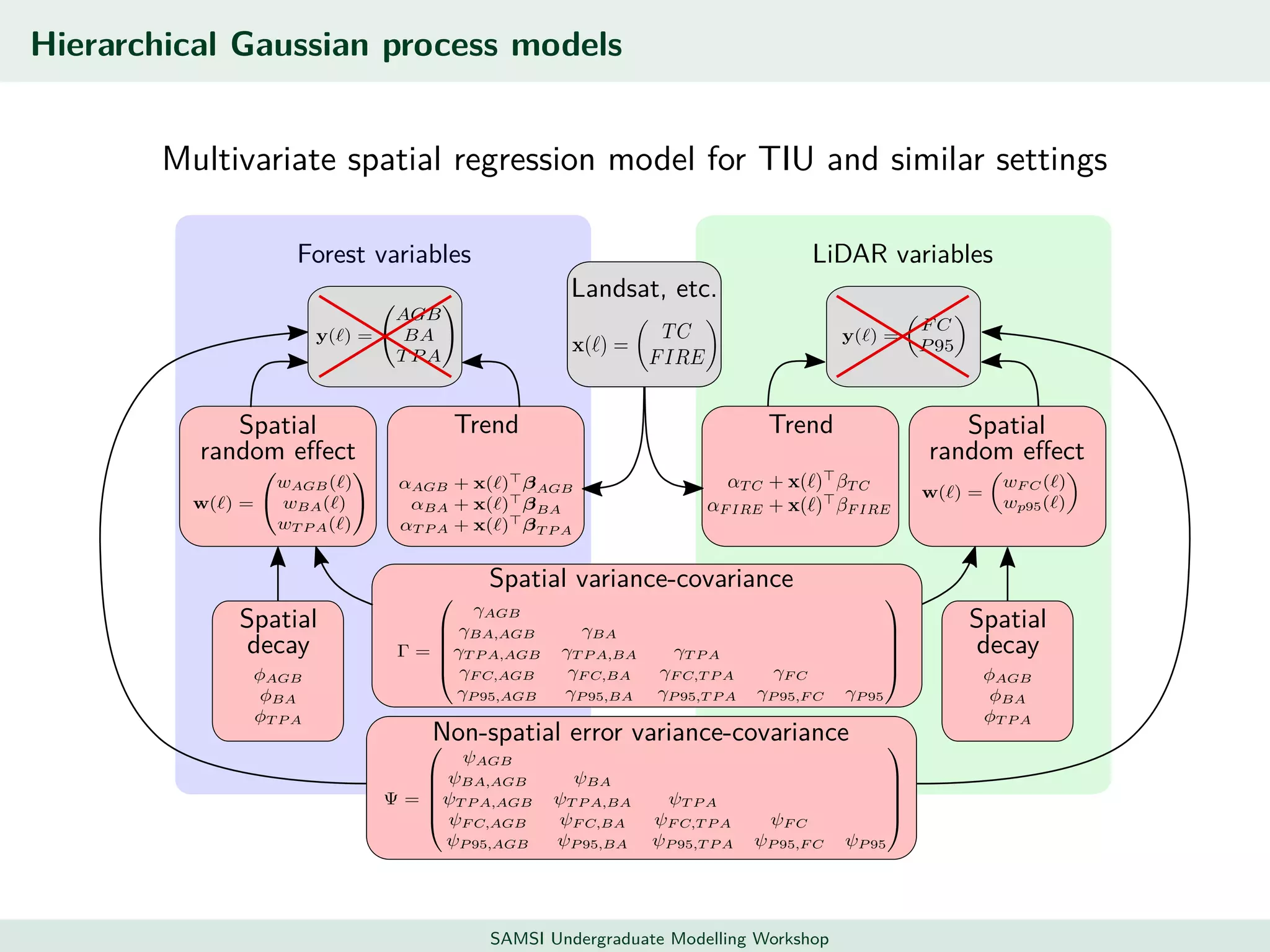
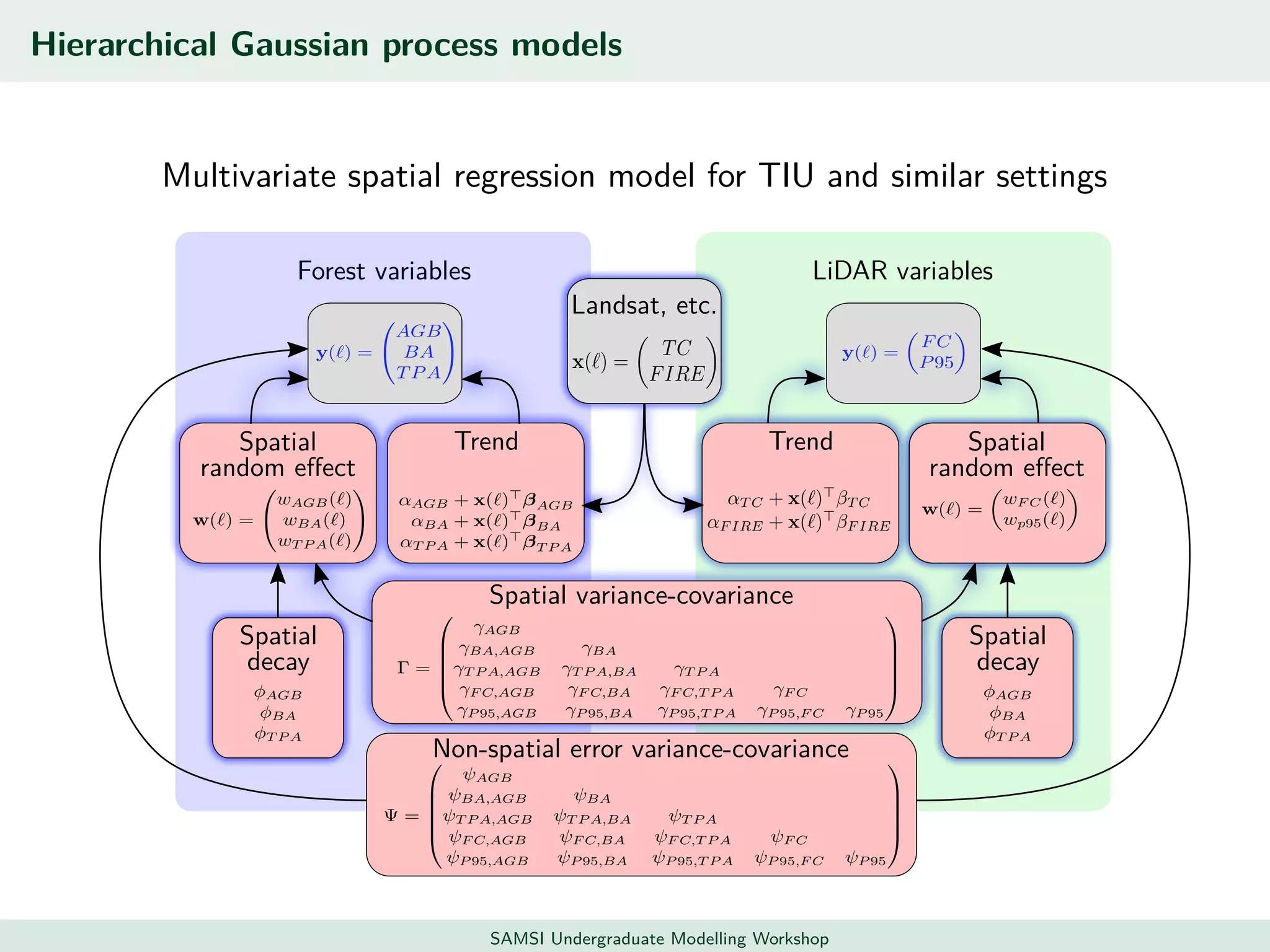
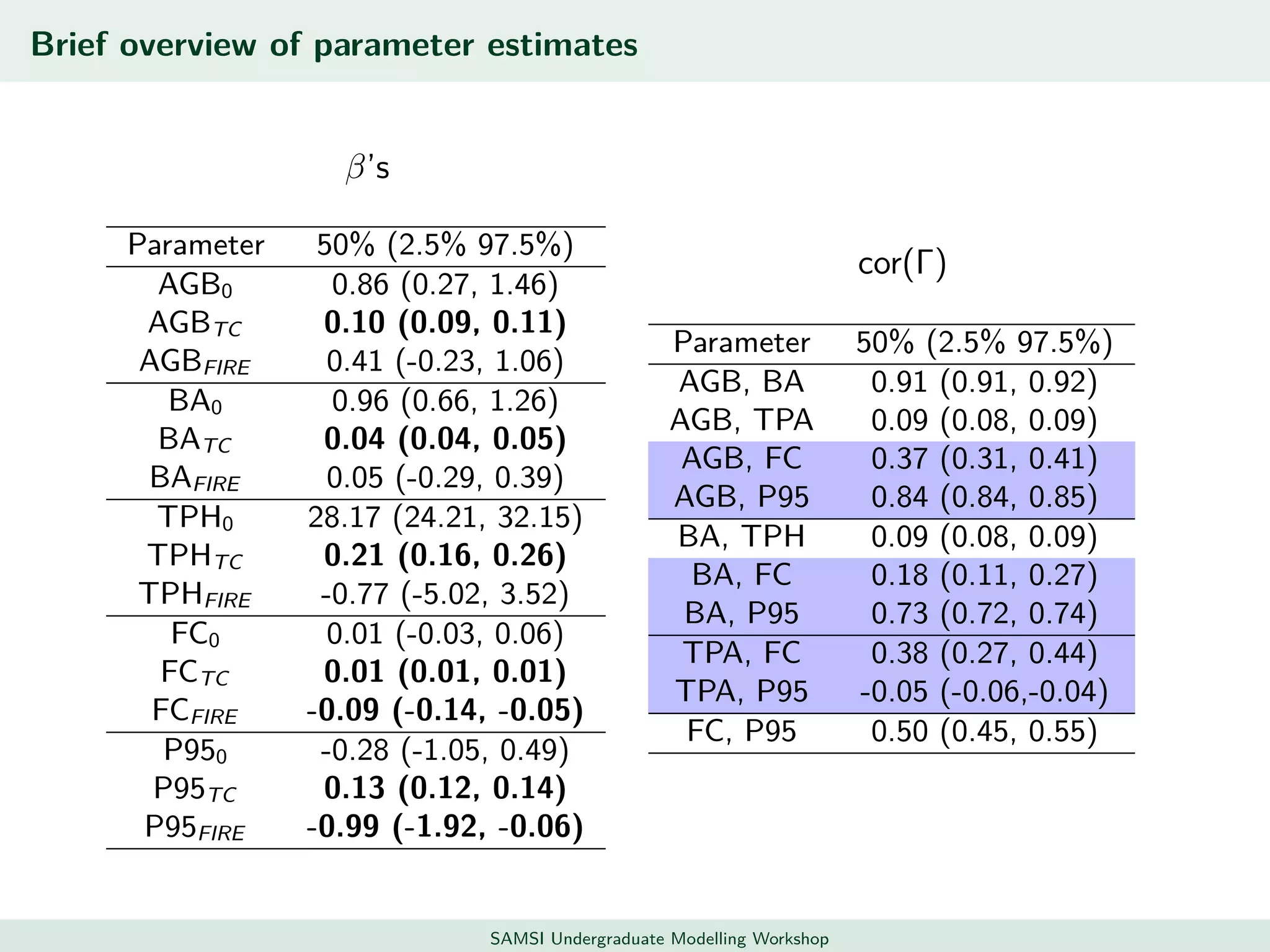
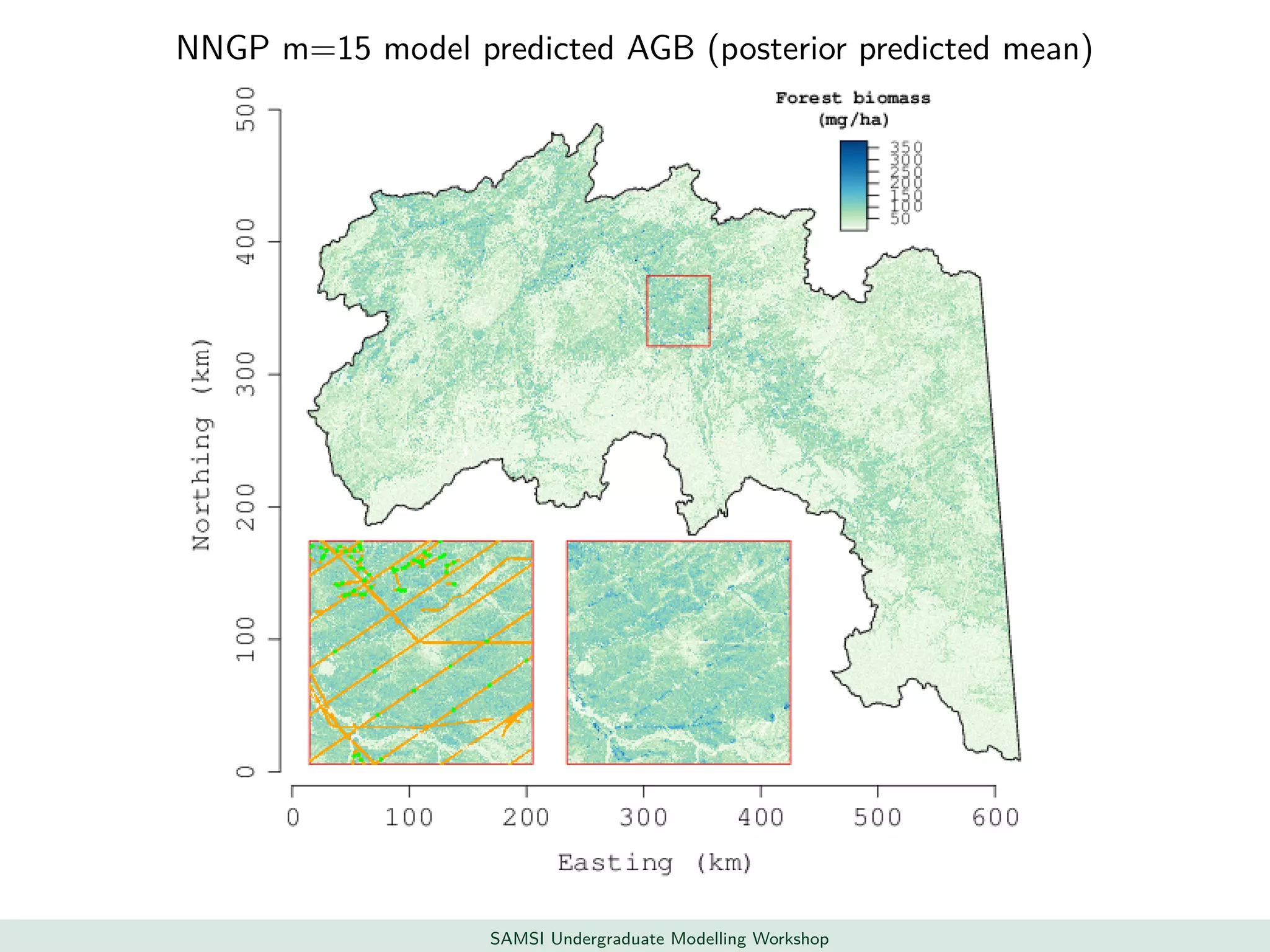
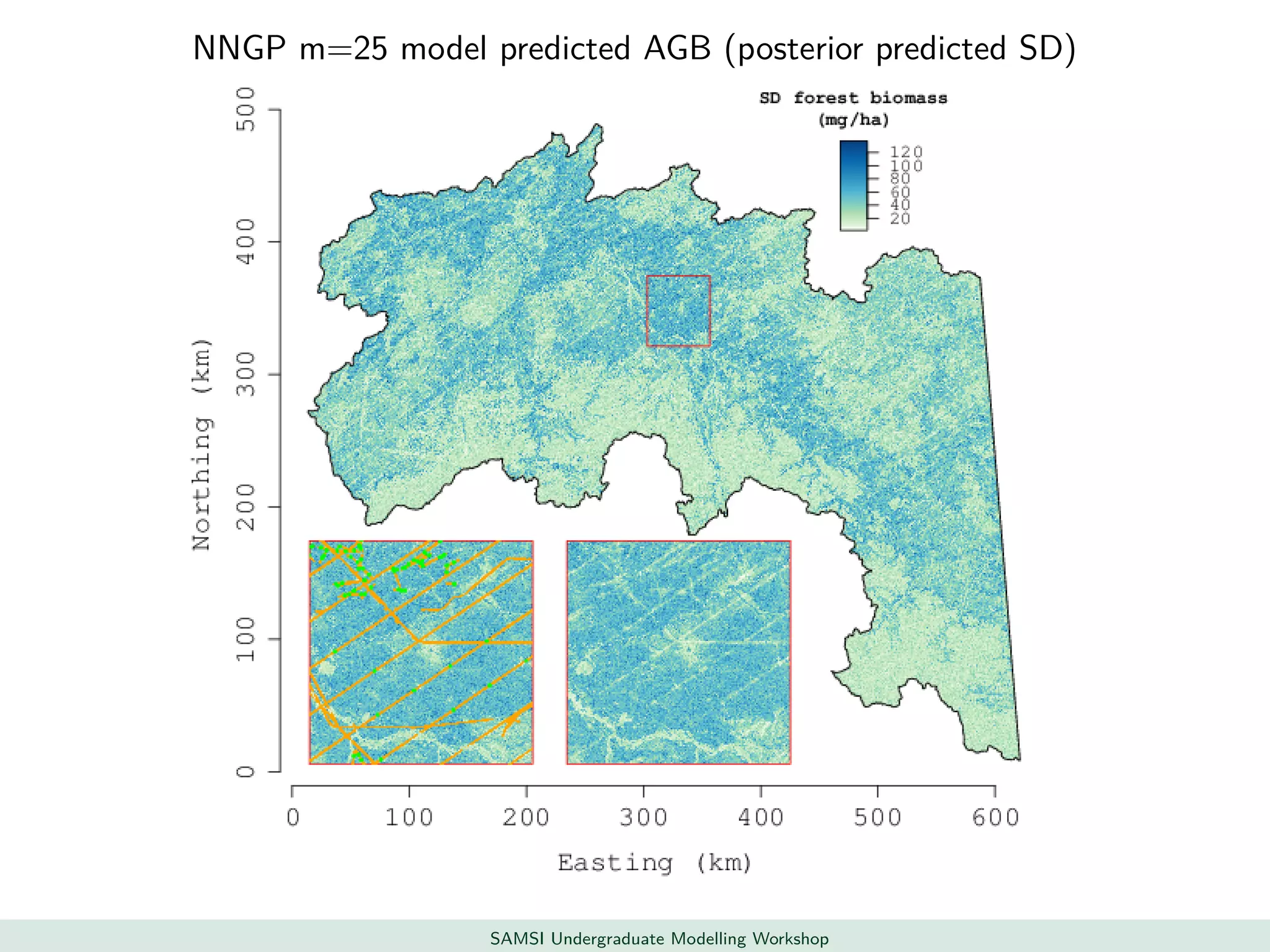
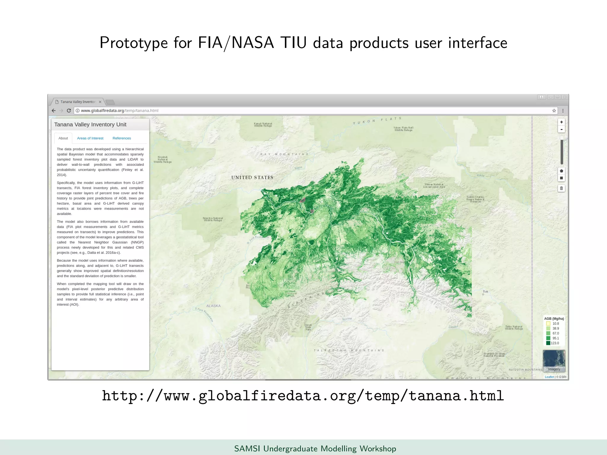
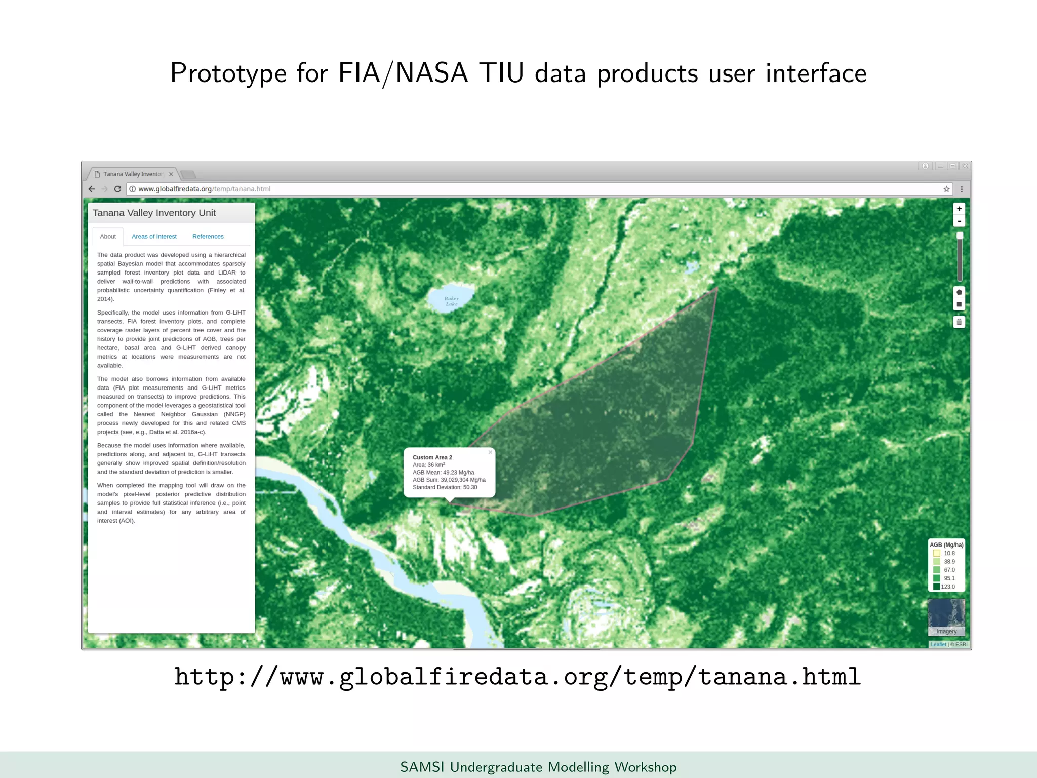
This document discusses challenges in analyzing large spatiotemporal environmental datasets and presents hierarchical Gaussian process models as a framework to address these challenges. It describes a joint NASA and Forest Service initiative applying these models to map forest variables in Interior Alaska using sparse ground plots and airborne/spaceborne LiDAR data. The key challenges are incorporating diverse spatial data sources, handling missingness/misalignment, accounting for spatial dependence, propagating uncertainty, and scaling to massive datasets.